
As discussed at the beginning of this chapter, instrumentation safety may be broadly divided into two categories: the safety hazards posed by malfunctioning instruments, and special instrument systems designed to reduce safety hazards of industrial processes. This section regards the first category.
All methods of reliability improvement incur some extra cost on the operation, whether it be capital expense (initial purchase/installation cost) or continuing expense (labor or consumables). The choice to improve system reliability is therefore very much an economic one. One of the human challenges associated with reliability improvement is continually justifying this cost over time. Ironically, the more successful a reliability improvement program has been, the less important that program seems. The manager of an operation suffering from reliability problems does not need to be convinced of the economic benefit of reliability improvement as much as the manager of a trouble-free facility. Furthermore, the people most aware of the benefits of reliability improvement are usually those tasked with reliability-improving duties (such as preventive maintenance), while the people least aware of the same benefits are usually those managing budgets. If ever a disagreement erupts between the two camps, pleas for continued financial support of reliability improvement programs may be seen as nothing more than self-interest, further escalating tensions23 .
A variety of methods exist to improve the reliability of systems. The following subsections investigate several of them.
32.4.1 Design and selection for reliability
Many workable designs may exist for electronic and mechanical systems alike, but not all are equal in terms of reliability. A major factor in machine reliability, for example, is balance. A well-balanced machine will operate with little vibration, whereas an ill-balanced machine will tend to shake itself (and other devices mechanically coupled to it) apart over time24 .
Electronic circuit reliability is strongly influenced by design as well as by component choice. An historical example of reliability-driven design is found in the Foxboro SPEC 200 analog control system. The reliability of the SPEC 200 control system is legendary, with a proven record of minimal failures over many years of industrial use. According to Foxboro technical literature, several design guidelines were developed following application experience with Foxboro electronic field instruments (most notably the “E” and “H” model lines), among them the following:
- All critical switches should spend most of their time in the closed state
- Avoid the use of carbon composition resistors – use wirewound or film-type resistors instead
- Avoid the use of plastic-cased semiconductors – use glass-cased or hermetically sealed instead
- Avoid the use of electrolytic capacitors wherever possible – use polycarbonate or tantalum instead
Each of these design guidelines is based on minimization of component failure. Having switches spend most of their lives in the closed state means their contact surfaces will be less exposed to air and therefore less susceptible to corrosion over time (leading to an “open” fault). Wirewound resistors are better able to tolerate vibration and physical abuse than brittle carbon-composition designs. Glass-cased and hermetically-sealed semiconductors are better at sealing out moisture than plastic-cased semiconductors. Electrolytic capacitors are famously unreliable compared to other capacitor types such as polycarbonate, and so their avoidance is wise.
In addition to high-quality component characteristics and excellent design practices, components used in these lines of Foxboro instruments were “burned in” prior to circuit board assembly, thus avoiding many “early failures” due to components “burning in” during actual service.
32.4.2 Preventive maintenance
The term preventive maintenance refers to the maintenance (repair or replacement) of components prior to their inevitable failure in a system. In order to intelligently schedule the replacement of critical system components, some knowledge of those components’ useful lifetimes is necessary. On the standard “bathtub curve,” this corresponds with the wear-out time or twear−out.
In many industrial operations, preventive maintenance schedules (if they exist at all) are based on past history of component lifetimes, and the operational expenses incurred due to failure of those components. Preventive maintenance represents an up-front cost, paid in exchange for the avoidance of larger costs later in time.
A common example of preventive maintenance and its cost savings is the periodic replacement of lubricating oil and oil filters for automobile engines. Automobile manufacturers provide specifications for the replacement of oil and filters based on testing of their engines, and assumptions made regarding the driving habits of their customers. Some manufacturers even provide dual maintenance schedules, one for “normal” driving and another for “heavy” or “performance” driving to account for accelerated wear. As trivial as an oil change might seem to the average driver, regular maintenance to an automobile’s lubrication system is absolutely critical not only to long service life, but also to optimum performance. Certainly, the consequences of not performing this preventive maintenance task on an automobile’s engine will be costly25 .
Another example of preventive maintenance for increased system reliability is the regular replacement of light bulbs in traffic signal arrays. For rather obvious reasons, the proper function of traffic signal lights is critical for smooth traffic flow and public safety. It would not be a satisfactory state of affairs to replace traffic signal light bulbs only when they failed, as is common with the replacement of most light bulbs. In order to achieve high reliability, these bulbs must be replaced in advance of their expected wear-out times26 . The cost of performing this maintenance is undeniable, but then so is the (greater) cost of congested traffic and accidents caused by burned-out traffic light bulbs.
An example of preventive maintenance in industrial instrumentation is the installation and service of dryer mechanisms for compressed air, used to power pneumatic instruments and valve actuators. Compressed air is a very useful medium for transferring (and storing) mechanical energy, but problems will develop within pneumatic instruments if water is allowed to collect within air distribution systems. Corrosion, blockages, and hydraulic “locking” are all potential consequences of “wet” instrument air. Consequently, instrument compressed air systems are usually installed separate from utility compressed air systems (used for operating general-purpose pneumatic tools and equipment actuators), using different types of pipe (plastic, copper, or stainless steel rather than black iron or galvanized iron) to avoid corrosion and using air dryer mechanisms near the compressor to absorb and expel moisture. These air dryers typically use a beaded desiccant material to absorb water vapor from the compressed air, and then this desiccant material is periodically purged of its retained water. After some time of operation, though, the desiccant must be physically removed and replaced with fresh desiccant.
32.4.3 Component de-rating
Some27 control system components exhibit an inverse relationship between service load (how “hard” the component is used) and service life (how long it will last). In such cases, a way to increase service life is to de-rate that component: operate it at a load reduced from its design rating.
For example, a variable-frequency motor drive (VFD) takes AC power at a fixed frequency and voltage and converts it into AC power of varying frequency and voltage to drive an induction motor at different speeds and torques. These electronic devices dissipate some heat owing mostly to the imperfect (slightly resistive) “on” states of power transistors. Temperature is a wear factor for semiconductor devices, with greater temperatures leading to reduced service lives. A VFD operating at high temperature, therefore, will fail sooner than a VFD operating at low temperature, all other factors being equal. One way to reduce the operating temperature of a VFD is to over-size it for the application. If the motor to be driven requires 2 horsepower of electrical power at full load, and increased reliability is demanded of the drive, then perhaps a 5 horsepower VFD (programmed with reduced trip settings appropriate to the smaller motor) could be chosen to drive the motor.
In addition to extending service life, de-rating also has the ability to amplify the mean time between failure (MTBF) of load-sensitive components. Recall that MTBF is the reciprocal of failure rate during the low area of the “bathtub curve,” representing failures due to random causes. This is distinct from wear-out, which is an increase in failure rate due to irreversible wear and aging. The main reason a component will exhibit a greater MTBF value as a consequence of de-rating is that the component will be better able to absorb transient overloads, which is a typical cause of failure during the operational life of system components.
Consider the example of a pressure sensor in a process known to exhibit transient pressure surges. A sensor chosen such that the typical process operating pressure spans most of its range will have little overpressure capacity. Perhaps just a few over-pressure events will cause this sensor to fail well before its rated service life. A de-rated pressure sensor (with a pressure-sensing range covering much greater pressures than what are normally encountered in this process), by comparison, will have more pressure capacity to withstand random surges, and therefore exhibit less probability of random failure.
The costs associated with component de-rating include initial investment (usually greater, owing to the greater capacity and more robust construction compared to a “normally” rated component) and reduced sensitivity. The latter factor is an important one to consider if the component is expected to provide high accuracy as well as high reliability. In the example of the de-rated pressure sensor, accuracy will likely suffer because the full pressure range of the sensor is not being used for normal process pressure measurements. If the instrument is digital, resolution will certainly suffer as a result of de-rating the instrument’s measurement range. Alternative methods of reliability improvement (including more frequent preventive maintenance) may be a better solution than de-rating in such cases.
32.4.4 Redundant components
The MTBF of any system dependent upon certain critical components may be extended by duplicating those components in parallel fashion, such that the failure of only one does not compromise the system as a whole. This is called redundancy. A common example of component redundancy in instrumentation and control systems is the redundancy offered by distributed control systems (DCSs), where processors, network cables, and even I/O (input/output) channels may be equipped with “hot standby” duplicates ready to assume functionality in the event the primary component fails.
Redundancy tends to extend the MTBF of a system without necessarily extending its service life. A DCS, for example, equipped with redundant microprocessor control modules in its rack, will exhibit a greater MTBF because a random microprocessor fault will be covered by the presence of the spare (“hot standby”) microprocessor module. However, given the fact that both microprocessors are continually powered, and therefore tend to “wear” at the same rate, their operating lives will not be additive. In other words, two microprocessors will not function twice as long before wear-out than one microprocessor.
The extension of MTBF resulting from redundancy holds true only if the random failures are truly independent events – that is, not associated by a common cause. To use the example of a DCS rack with redundant microprocessor control modules again, the susceptibility of that rack to a random microprocessor fault will be reduced by the presence of redundant microprocessors only if the faults in question are unrelated to each other, affecting the two microprocessors separately. There may exist common-cause fault mechanisms capable of disabling both microprocessor modules as easily as it could disable one, in which case the redundancy adds no value at all. Examples of such common-cause faults include power surges (because a surge strong enough to kill one module will likely kill the other at the same time) and a computer virus infection (because a virus able to attack one will be able to attack the other just as easily, and at the same time).
A simple example of component redundancy in an industrial instrumentation system is dual DC power supplies feeding through a diode module. The following photograph shows a typical example, in this case a pair of Allen-Bradley AC-to-DC power supplies for a DeviceNet digital network:
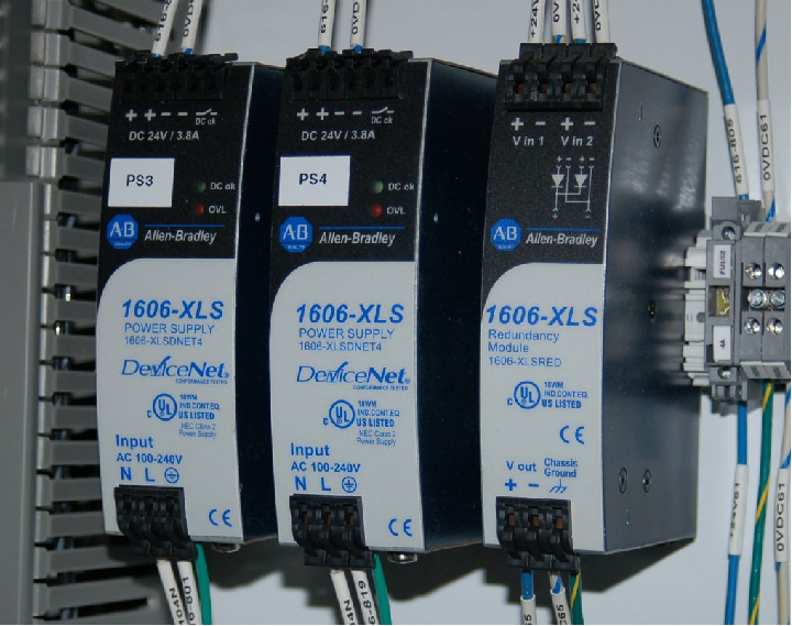
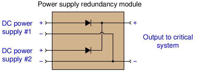
If either of the two AC-to-DC power supplies happens to fail with a low output voltage, the other power supply is able to carry the load by passing its power through the diode redundancy module28 :
In order for redundant components to actually increase system MTBF, the potential for common-cause failures must be addressed. For example, consider the effects of powering redundant AC-to-DC power supplies from the exact same AC line. Redundant power supplies would increase system reliability in the face of a random power supply failure, but this redundancy would do nothing at all to improve system reliability in the event of the common AC power line failing! In order to enjoy the fullest benefit of redundancy in this example, we must source each AC-to-DC power supply from a different (unrelated) AC line.
Another example of redundancy in industrial instrumentation is the use of multiple transmitters to sense the same process variable, the notion being that the critical process variable will still be monitored even in the event of a transmitter failure. Thus, installing redundant transmitters should increase the MTBF of the system’s sensing ability.
Here again, we must address common-cause failures in order to reap the full benefits of redundancy. If three liquid level transmitters are installed to measure the exact same liquid level, their combined signals represent an increase in measurement system MTBF only for independent faults. A failure mechanism common to all three transmitters will leave the system just as vulnerable to random failure as a single transmitter. In order to achieve optimum MTBF in redundant sensor arrays, the sensors must be immune to common faults.
In this example, three different types of level transmitter monitor the level of liquid inside a vessel, their signals processed by a selector function programmed inside a DCS:
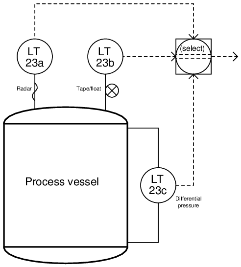
Here, level transmitter 23a is a guided-wave radar (GWR), level transmitter 23b is a tape-and-float, and level transmitter 23c is a differential pressure sensor. All three level transmitters sense liquid level using different technologies, each one with its own strengths and weaknesses. Better redundancy of measurement is obtained this way, since no single process condition or other random event is likely to fault more than one of the transmitters at any given time.
For instance, if the process liquid density happened to suddenly change, it would affect the measurement accuracy of the differential pressure transmitter (LT-23c), but not the radar transmitter nor the tape-and-float transmitter. If the process vapor density were to suddenly change, it might affect the radar transmitter (since vapor density generally affects dielectric constant, and dielectric constant affects the propagation velocity of electromagnetic waves, which in turn will affect the time taken for the radar pulse to strike the liquid surface and return), but this will not affect the float transmitter’s accuracy nor will it affect the differential pressure transmitter’s accuracy. Surface turbulence of the liquid inside the vessel may severely affect the float transmitter’s ability to accurately sense liquid level, but it will have little effect on the differential pressure transmitter’s reading nor the radar transmitter’s measurement (assuming the radar transmitter is shrouded in a stilling well.
If the selector function takes either the median (middle) measurement or an average of the best 2-out-of-3 (“2oo3”), none of these random process occurrences will greatly affect the selected measurement of liquid level inside the vessel. True redundancy is achieved here, since the three level transmitters are not only less likely to (all) fail simultaneously than for any single transmitter to fail, but also because the level is being sensed in three completely different ways.
A crucial requirement for redundancy to be effective is that all redundant components must have precisely the same process function. In the case of redundant DCS components such as processors, I/O cards, and network cables, each of these redundant components must do nothing more than serve as “backup” spares for their primary counterparts. If a particular DCS node were equipped with two processors – one as the primary and another as a secondary (backup) – but yet the backup processor were tasked with some detail specific to it and not to the primary processor (or vice-versa), the two processors would not be truly redundant to each other. If one processor were to fail, the other would not perform exactly the same function, and so the system’s operation would be affected (even if only in a small way) by the processor failure.
Likewise, redundant sensors must perform the exact same process measurement function in order to be truly redundant. A process equipped with triplicate measurement transmitters such as the previous example were a vessel’s liquid level was being measured by a guided-wave radar, tape-and-float, and differential pressure based level transmitters, would enjoy the protection of redundancy if and only if all three transmitters sensed the exact same liquid level over the exact same calibrated range. This often represents a challenge, in finding suitable locations on the process vessel for three different instruments to sense the exact same process variable. Quite often, the pipe fittings penetrating the vessel (often called nozzles) are not conveniently located to accept multiple instruments at the points necessary to ensure consistency of measurement between them. This is often the case when an existing process vessel is retrofitted with redundant process transmitters. New construction is usually less of a problem, since the necessary nozzles and other accessories may be placed in their proper positions during the design stage29 .
If fluid flow conditions inside a process vessel are excessively turbulent, multiple sensors installed to measure the same variable will sometimes report significant differences. Multiple temperature transmitters located in close proximity to each other on a distillation column, for example, may report significant differences of temperature if their respective sensing elements (thermocouples, RTDs) contact the process liquid or vapor at points where the flow patterns vary. Multiple liquid level sensors, even of the same technology, may report differences in liquid level if the liquid inside the vessel swirls or “funnels” as it enters and exits the vessel.
Not only will substantial measurement differences between redundant transmitters compromise their ability to function as “backup” devices in the event of a failure, such differences may actually “fool” a redundant system into thinking one or more of the transmitters has already failed, thereby causing the deviating measurement to be ignored. To use the triplicate level-sensing array as an example again, suppose the radar-based level transmitter happened to register two inches greater level than the other two transmitters due to the effects30 of liquid swirl inside the vessel. If the selector function is programmed to ignore such deviating measurements, the system degrades to a duplicate-redundant instead of triplicate-redundant array. In the event of a dangerously low liquid level, for example, only the radar-based and float-based level transmitters will be ready to signal this dangerous process condition to the control system, because the pressure-based level transmitter is registering too high.
32.4.5 Proof tests and self-diagnostics
A reliability enhancing technique related to preventive maintenance of critical instruments and functions, but generally not as expensive as component replacement, is periodic testing of component and system function. Regular “proof testing” of critical components enhances the MTBF of a system for two different reasons:
- Early detection of developing problems
- Regular “exercise” of components
First, proof testing may reveal weaknesses developing in components, indicating the need for replacement in the near future. An analogy to this is visiting a doctor to get a comprehensive exam – if this is done regularly, potentially fatal conditions may be detected early and crises averted.
The second way proof testing increases system reliability is by realizing the beneficial effects of regular function. The performance of many component and system types tends to degrade after prolonged periods of inactivity31 . This tendency is most prevalent in mechanical systems, but holds true for some electrical components and systems as well. Solenoid valves, for instance, may become “stuck” in place if not cycled for long periods of time. Bearings may corrode and seize in place if left immobile. Both primary- and secondary-cell batteries are well known for their tendency to fail after prolonged periods of non-use. Regular cycling of such components actually enhances their reliability, decreasing the probability of a “stagnation” related failure well before the rated useful life has elapsed.
An important part of any proof-testing program is to ensure a ready stock of spare components is kept on hand in the event proof-testing reveals a failed component. Proof testing is of little value if the failed component cannot be immediately repaired or replaced, and so these warehoused components should be configured (or be easily configurable) with the exact parameters necessary for immediate installation. A common tendency in business is to focus attention on the engineering and installation of process and control systems, but neglect to invest in the support materials and infrastructure to keep those systems in excellent condition. High-reliability systems have special needs, and this is one of them.
Methods of proof testing
The most direct method of testing a critical system is to stimulate it to its range limits and observe its reaction. For a process transmitter, this sort of test usually takes the form of a full-range calibration check. For a controller, proof testing would consist of driving all input signals through their respective ranges in all combinations to check for the appropriate output response(s). For a final control element (such as a control valve), this requires full stroking of the element, coupled with physical leakage tests (or other assessments) to ensure the element is having the intended effect on the process.
An obvious challenge to proof testing is how to perform such comprehensive tests without disrupting the process in which it functions. Proof-testing an out-of-service instrument is a simple matter, but proof-testing an instrument installed in a working system is something else entirely. How can transmitters, controllers, and final control elements be manipulated through their entire operating ranges without actually disturbing (best case) or halting (worst case) the process? Even if all tests may be performed at the required intervals during shut-down periods, the tests are not as realistic as they could be with the process operating at typical pressures and temperatures. Proof-testing components during actual “run” conditions is the most realistic way to assess their readiness.
One way to proof-test critical instruments with minimal impact to the continued operation of a process is to perform the tests on only some components, not all. For instance, it is a relatively simple matter to take a transmitter out of service in an operating process to check its response to stimuli: simply place the controller in manual mode and let a human operator control the process manually while an instrument technician tests the transmitter. While this strategy admittedly is not comprehensive, at least proof-testing some of the instruments is better than proof-testing none of them.
Another method of proof-testing is to “test to shutdown:” choose a time when operations personnel plan on shutting the process down anyway, then use that time as an opportunity to proof-test one or more critical component(s) necessary for the system to run. This method enjoys the greatest degree of realism, while avoiding the inconvenience and expense of an unnecessary process interruption.
Yet another method to perform proof tests on critical instrumentation is to accelerate the speed of the testing stimuli so that the final control elements will not react fully enough to actually disrupt the process, but yet will adequately assess the responsiveness of all (or most) of the components in question. The nuclear power industry sometimes uses this proof-test technique, by applying high-speed pulse signals to safety shutdown sensors in order to test the proper operation of shutdown logic, without actually shutting the reactor down. The test consists of injecting short-duration pulse signals at the sensor level, then monitoring the output of the shutdown logic to ensure consequent pulse signals are sent to the shutdown device(s). Various chemical and petroleum industries apply a similar proof-testing technique to safety valves called partial stroke testing, whereby the valve is stroked only part of its travel: enough to ensure the valve is capable of adequate motion without closing (or opening, depending on the valve function) enough to actually disrupt the process.
Redundant systems offer unique benefits and challenges to component proof-testing. The benefit of a redundant system in this regard is that any one redundant component may be removed from service for testing without any special action by operations personnel. Unlike a “simplex” system where removal of an instrument requires a human operator to manually take over control during the duration of the test, the “backup” components of a redundant system should do this automatically, theoretically making the test much easier to conduct. However, the challenge of doing this is the fact that the portion of the system responsible for ensuring seamless transition in the event of a failure is in fact a component liable to failure itself. The only way to test this component is to actually disable one (or more, in highly redundant configurations) of the redundant components to see whether or not the remaining component(s) perform their redundant roles. So, proof-testing a redundant system harbors no danger if all components of the system are good, but risks process disruption if there happens to be an undetected fault.
Let us return to our triplicate level transmitter system once again to explore these concepts. Suppose we wished to perform a proof-test of the pressure-based level transmitter. Being one of three transmitters measuring liquid level in this vessel, we should be able to remove it from service with no preparation (other than notifying operations personnel of the test, and of the potential consequences) since the selector function should automatically de-select the disabled transmitter and continue measuring the process via the remaining two transmitters. If the proof-testing is successful, it proves not only that the transmitter works, but also that the selector function adequately performed its task in “backing up” the tested transmitter while it was removed. However, if the selector function happened to be failed when we disable the one level transmitter for proof-testing, the selected process level signal could register a faulty value instead of switching to the two remaining transmitters’ signals. This might disrupt the process, especially if the selected level signal went to a control loop or to an automatic shutdown system. We could, of course, proceed with the utmost caution by having operations personnel place the control system in “manual” mode while we remove that one transmitter from service, just in case the redundancy does not function as designed. Doing so, however, fails to fully test the system’s redundancy, since by placing the system in manual mode before the test we do not allow the redundant logic to fully function as it would be expected to in the event of an actual instrument failure.
Regular proof-testing is an essential activity to realize optimum reliability for any critical system. However, in all proof-testing we are faced with a choice: either test the components to their fullest degree, in their normal operating modes, and risk (or perhaps guarantee) a process disruption; or perform a test that is less than comprehensive, but with less (or no) risk of process disruption. In the vast majority of cases, the latter option is chosen simply due to the costs associated with process disruption. Our challenge as instrumentation professionals is to formulate proof tests that are as comprehensive as possible while being the least disruptive to the process we are trying to regulate.
Instrument self-diagnostics
One of the great advantages of digital electronic technology in industrial instrumentation is the inclusion of self-diagnostic ability in field instruments. A “smart” instrument containing its own microprocessor may be programmed to detect certain conditions known to indicate sensor failure or other problems, then signal the control system that something is wrong. Though self-diagnostics can never be perfectly effective in that there will inevitably be cases of undetected faults and even false positives (declarations of a fault where none exists), the current state of affairs is considerably better than the days of purely analog technology where instruments possessed little or no self-diagnostic capability.
Digital field instruments have the ability to communicate self-diagnostic error messages to their host systems over the same “fieldbus” networks they use to communicate regular process data. FOUNDATION Fieldbus instruments in particular have extensive error-reporting capability, including a “status” variable associated with every process signal that propagates down through all function blocks responsible for control of the process. Detected faults are efficiently communicated throughout the information chain in the system when instruments have full digital communication ability.
“Smart” instruments with self-diagnostic ability but limited to analog (e.g. 4-20 mA DC) signaling may also convey error information, just not as readily or as comprehensively as a fully digital instrument. The NAMUR recommendations for 4-20 mA signaling (NE-43) provide a means to do this:
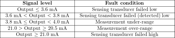
Proper interpretation of these special current ranges, of course, demands a receiver capable of accurate current measurement outside the standard 4-20 mA range. Many control systems with analog input capability are programmed to recognize the NAMUR error-indicating current levels.
A challenge for any self-diagnostic system is how to check for faults in the “brain” of the unit itself: the microprocessor. If a failure occurs within the microprocessor of a “smart” instrument – the very component responsible for performing logic functions related to self-diagnostic testing – how would it be able to detect a fault in logic? The question is somewhat philosophical, equivalent to determining whether or not a neurologist is able to diagnose his or her own neurological problems.
One simple method of detecting gross faults in a microprocessor system is known as a watchdog timer. The principle works like this: the microprocessor is programmed to output continuous a low-frequency pulse signal, with an external circuit “watching” that pulse signal for any interruptions or freezing. If the microprocessor fails in any significant way, the pulse signal will either skip pulses or “freeze” in either the high or low state, thus indicating a microprocessor failure to the “watchdog” circuit.
One may construct a watchdog timer circuit using a pair of solid-state timing relays connected to the pulse output channel of the microprocessor device:
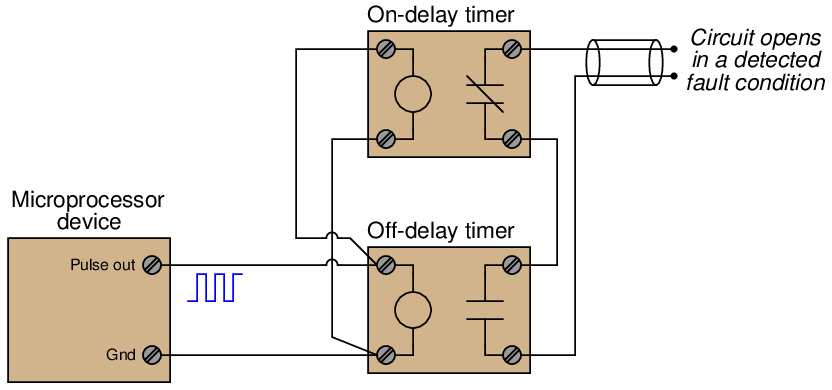
Both the on-delay and off-delay timers receive the same pulse signal from the microprocessor, their inputs connected directly in parallel with the microprocessor’s pulse output. The off-delay timer immediately actuates upon receiving a “high” signal, and begins to time when the pulse signal goes “low.” The on-delay timer begins to time during a “high” signal, but immediately de-actuates whenever the pulse signal goes “low.” So long as the time settings for the on-delay and off-delay timer relays are greater than the “high” and “low” durations of the watchdog pulse signal, respectively, neither relay contact will open as long as the pulse signal continues in its regular pattern.
When the microprocessor is behaving normally, outputting a regular watchdog pulse signal, the off-delay timer’s contact will hold in a closed state because it keeps getting energized with each “high” signal and never has enough time to drop out during each “low” signal. Likewise, the on-delay timer’s contact will remain in its normally closed state because it never has enough time to pick up during each “high” signal before being de-actuated with each “low” signal. Both timing relay contacts will be in a closed state when all is well.
However, if the microprocessor’s pulse output signal happens to freeze in the “low” state (or skip a “high” pulse), the off-delay timer will de-actuate, opening its contact and signaling a fault. Conversely, if the microprocessor’s pulse signal happens to freeze in the “high” state (or skip a “low” pulse), the on-delay timer will actuate, opening its contact and signaling a fault. Either timing relay opening its contact signals an interruption or cessation of the watchdog pulse signal, indicating a serious microprocessor fault