
Flow, by definition, is the passage of material from one location to another over time. So far this chapter has explored technologies for measuring flow rate en route from source to destination. However, a completely different method exists for measuring flow rates: measuring how much material has either departed or arrived at the terminal locations over time.
Mathematically, we may express flow as a ratio of quantity to time. Whether it is volumetric flow or mass flow we are referring to, the concept is the same: quantity of material moved per quantity of time. We may express average flow rates as ratios of changes:
Where,
W = Average mass flow rate
Q = Average volumetric flow rate
Δm = Change in mass
ΔV = Change in volume
Δt = Change in time
Suppose a water storage vessel is equipped with load cells to precisely measure weight (which is directly proportional to mass with constant gravity). Assuming only one pipe entering or exiting the vessel, any flow of water through that pipe will result in the vessel’s total weight changing over time:
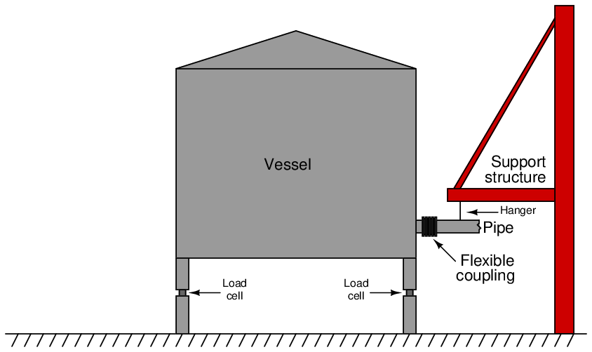
If the measured mass of this vessel decreased from 74688 kilograms to 70100 kilograms between 4:05 AM and 4:07 AM, we could say that the average mass flow rate of water leaving the vessel is 2294 kilograms per minute over that time span.

Note that this average flow measurement may be determined without any flowmeter of any kind installed in the pipe to intercept the water flow. All the concerns of flowmeters studied thus far (turbulence, Reynolds number, fluid properties, etc.) are completely irrelevant. We may measure practically any flow rate we desire simply by measuring stored weight (or volume) over time. A computer may do this calculation automatically for us if we wish, on practically any time scale desired.
Now suppose the practice of determining average flow rates every two minutes was considered too infrequent. Imagine that operations personnel require flow data calculated and displayed more often than just 30 times an hour. All we must do to achieve better time resolution is take weight (mass) measurements more often. Of course, each mass-change interval will be expected to be less with more frequent measurements, but the amount of time we divide by in each calculation will be proportionally smaller as well. If the flow rate happens to be absolutely steady, we may sample mass as frequently as we might like and we will still arrive at the same flow rate value as before (sampling mass just once every two minutes). If, however, the flow rate is not steady, sampling more often will allow us to better see the immediate “ups” and “downs” of flow behavior.
Imagine now that we had our hypothetical “flow computer” take weight (mass) measurements at an infinitely fast pace: an infinite number of samples per second. Now, we are no longer averaging flow rates over finite periods of time; instead we would be calculating instantaneous flow rate at any given point in time.
Calculus has a special form of symbology to represent such hypothetical scenarios: we replace the Greek letter “delta” (Δ, meaning “change”) with the roman letter “d” (meaning differential). A simple way of picturing the meaning of “d” is to think of it as meaning an infinitesimal change in whatever variable follows the “d” in the equation78 . When we set up two differentials in a quotient, we call the d d fraction a derivative. Re-writing our average flow rate equations in derivative (calculus) form:
Where,
W = Instantaneous mass flow rate
Q = Instantaneous volumetric flow rate
dm = Infinitesimal (infinitely small) change in mass
dV = Infinitesimal (infinitely small) change in volume
dt = Infinitesimal (infinitely small) change in time
We need not dream of hypothetical computers capable of infinite calculations per second in order to derive a flow measurement from a mass (or volume) measurement. Analog electronic circuitry exploits the natural properties of resistors and capacitors to essentially do this very thing in real time79 :
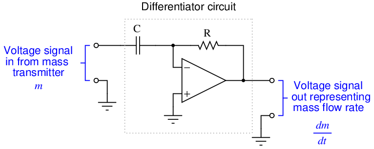
In the vast majority of applications you will see digital computers used to calculate average flow rates rather than analog electronic circuits calculating instantaneous flow rates. The broad capabilities of digital computers virtually ensures they will be used somewhere in the measurement/control system, so the rationale is to use the existing digital computer to calculate flow rates (albeit imperfectly) rather than complicate the system design with additional (analog) circuitry. As fast as modern digital computers are able to process simple calculations such as these anyway, there is little practical reason to prefer analog signal differentiation except in specialized applications where high speed performance is paramount.
Perhaps the single greatest disadvantage to inferring flow rate by differentiating mass or volume measurements over time is the requirement that the storage vessel have only one flow path in and out. If the vessel has multiple paths for liquid to move in and out (simultaneously), any flow rate calculated on change-in-quantity will be a net flow rate only. It is impossible to use this flow measurement technique to measure one flow out of multiple flows common to one liquid storage vessel.
A simple “thought experiment” confirms this fact. Imagine a water storage vessel receiving a flow rate in at 200 gallons per minute. Next, imagine that same vessel emptying water out of a second pipe at the exact same flow rate: 200 gallons per minute. With the exact same flow rate both entering and exiting the vessel, the water level in the vessel will remain constant. Any change-of-quantity flow measurement system would register zero change in mass or volume over time, consequently calculating a flow rate of absolutely zero. Truly, the net flow rate for this vessel is zero, but this tells us nothing about the flow in each pipe, except that those flow rates are equal in magnitude and opposite in direction.