
Calculus has a reputation for being difficult to learn, and with good reason. The traditional approach to teaching calculus is based on manipulating symbols (variables) in equations, learning how different types of mathematical functions become transformed by the calculus operations of differentiation and integration.
For example, suppose a first-semester calculus student were given the following function to differentiate. The function is expressed as y in terms of x:
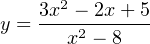
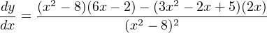
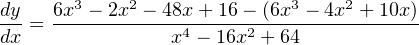
A calculus student would first apply two basic rules of symbolic differentiation (namely, the Power Rule and the Quotient Rule) followed by algebraic distribution and combination of like terms to arrive at the derivative of y with respect to x (written as dy dx) in terms of x:
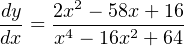
The resulting derivative expresses the rate-of-change of y with respect to x of the original function for any value of x. In other words, anyone can now plug any arbitrary value of x they wish into the derivative equation, and the result (dy/dx) will tell them how steep the slope is of the original function at that same x value10 .
Rules such as the Power Rule and even the Quotient Rule are not difficult to memorize, but they are far from intuitive. Although it is possible to formally prove each one of them from more fundamental principles of algebra, doing so is tedious, and so most students simply resign themselves to memorizing all the calculus rules of differentiation and integration. There are many such rules to memorize in symbolic calculus.
Symbolic integration is even more difficult to learn than symbolic differentiation. Most calculus textbooks reserve pages at the very end listing the general rules of differentiation and integration. Whereas a table of derivatives might occupy a single page in a calculus text, tables of integrals may fill five or more pages!
The next logical topic in the sequence of a calculus curriculum is differential equations. A “differential equation” is a function relating some variable to one or more of its own derivatives. To use the variables y and x, a differential equation would be one containing both y and at least one derivative of y (dy/dx, d2y/dx2 , d3y/dx3 , etc.). dV / dt = −kV is an example of a simple differential equation. The various forms and solution techniques for different kinds of differential equations are numerous and complex.
It has been said that the laws of the universe are written in the language of calculus. This is immediately evident in the study of physics, but it is also true for chemistry, biology, astronomy, and other “hard sciences.” Areas of applied science including engineering (chemical, electrical, mechanical, and civil) as well as economics, statistics, and genetics would be impoverished if not for the many practical applications of symbolic calculus. To be able to express a function of real-life quantities as a set of symbols, then apply the rules of calculus to those symbols to transform them into functions relating rates of change and accumulations of those real-life quantities, is an incredibly powerful tool.
Two significant problems exist with symbolic calculus, however. The first problem with symbolic calculus is its complexity, which acts as a barrier to many people trying to learn it. It is quite common for students to drop out of calculus or to change their major of study in college because they find the subject so confusing and/or frustrating. This is a shame, not only because those students end up missing out on the experience of being able to see the world around them in a new way, but also because mastery of calculus is an absolute requirement of entry into many professions. One cannot become a licensed engineer in the United States, for example, without passing a series of calculus courses in an accredited university and demonstrating mastery of those calculus concepts on a challenging exam.
The second significant problem with symbolic calculus is its limitation to a certain class of mathematical functions. In order to be able to symbolically differentiate a function (e.g. y = f(x)) to determine its derivative (dy/dx), we must first have a function written in mathematical symbols to differentiate. This rather obvious fact becomes a barrier when the data we have from a real-life application defies symbolic expression. It is trivial for a first-semester calculus student to determine the derivative of the function V = 2t2 − 4t + 9, but what if V and t only exist as recorded values in a table, or as a trend drawn by a process recorder? Without a mathematical formula showing V as a function of t, none of the rules learned in a calculus course for manipulating those symbols directly apply. The problem is even worse for differential equations, where a great many examples exist that have so far defied solution by the greatest mathematicians.
Such is the case when we apply calculus to recorded values of process variable, setpoint, and controller output in real-world automated processes. A trend showing a PV over time never comes complete with a formula showing you PV = f(t). We must approach these practical applications from some perspective other than symbolic manipulation if we are to understand how calculus relates. Students of instrumentation face this problem when learning PID control: the most fundamental algorithm of feedback control, used in the vast majority of industrial processes to regulate process variables to their setpoint values.
An alternative approach to calculus exists which is easily understood by anyone with the ability to perform basic arithmetic (addition, subtraction, multiplication, and division) and sketching (drawing lines and points on a graph). Numerical calculus uses simple arithmetic to approximate derivatives and integrals on real-world data. The results are not as precise as with symbolic calculus, but the technique works on any data as well as most mathematical functions written in symbolic form. Furthermore, the simplicity of these techniques opens a door to those people who might otherwise be scared away by the mathematical rigor of symbolic calculus. Any way we can find to showcase the beauty and practicality of calculus principles to more people is a good thing!
Suppose we needed to calculate the derivative of some real-world function, such as the volume of liquid contained in a storage vessel. The derivative of volume (V ) with respect to time (t) is volumetric flow rate (dV / dt ), thus the time-derivative of the vessel’s volume function at any specified point in time will be the net flow rate into (or out of) that vessel at that point in time.
To numerically determine the derivative of volume from raw data, we could follow these steps:
- Choose two values of volume both near the point in time we’re interesting in calculating flow rate.
- Subtract the two volume values: this will be ΔV .
- Subtract the two time values corresponding to those volume values: this will be Δt.
- Divide ΔV by Δt to approximate dV / dt between those two points in time.
A slightly different approach to numerical differentiation follows these steps:
- Sketch a graph of the volume versus time data for this vessel (if this has not already been done for you by a trend recorder).
- Locate the point in time on this graph you are interested in, and sketch a tangent line to that point (a straight line having the same slope as the graphed data at that point).
- Estimate the rise-over-run slope of this tangent line to approximate dV / dt at this point.
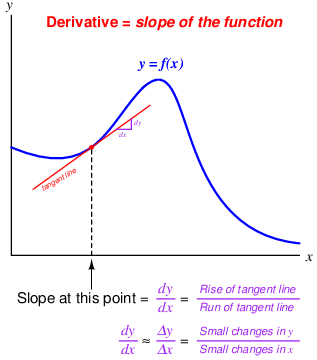
An illustration is a helpful reminder of what differentiation means for any graphed function: the slope of that function at a specified point:
Suppose we needed to calculate the integral of some real-world function, such as the flow rate of liquid through a pipe. The integral of volumetric flow (Q) with respect to time (t) is total volume (V ), thus the time-integral of the flow rate over any specified time interval will be the total volume of liquid that passed by over that time.
To numerically determine the integral of flow from raw data, we could follow these steps:
- Identify the time interval over which we intend to calculate volume, and the duration of each measured data point within that interval.
- Multiply each measured value of flow by the duration of that measurement (the interval between that measurement and the next one) to obtain a volume over each duration.
- Repeat the last step for each and every flow data point up to the end of the interval we’re interested in.
- Add all these volume values together – the result will be the approximate liquid volume passed through the pipe over the specified time interval.
A slightly different approach to numerical integration follows these steps:
- Sketch a graph of the flow versus time data for this pipe (if this has not already been done for you by a trend recorder).
- Mark the time interval over which we intend to calculate volume (two straight vertical lines on the graph).
- Use any geometrical means available to estimate the area bounded by the graph and the two vertical time markers – the result will be the approximate liquid volume passed through the pipe over the specified time interval.
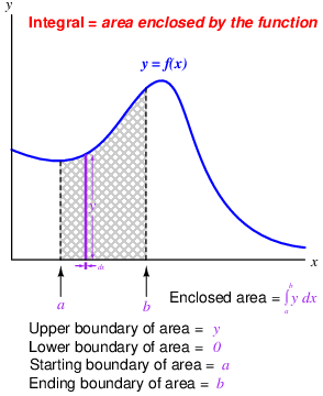
An illustration is a helpful reminder of what integration means for any graphed function: the area enclosed by that function within a specified set of boundaries:
The next sections of this chapter delve into more specific details of numerical differentiation and integration, with realistic examples to illustrate.