
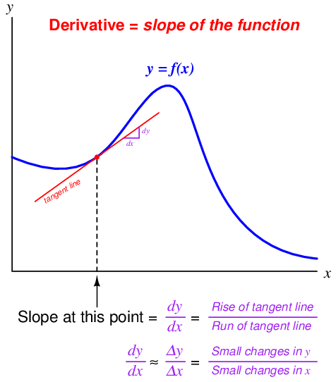
First, let us review some of the properties of differentials and derivatives, referencing the expression and graph shown below:
- A differential is an infinitesimal increment of change (difference) in some continuously-changing variable, represented either by a lower-case Roman letter d or a lower-case Greek letter “delta” (δ). Such a change in time would be represented as dt; a similar change in temperature as dT; a similar change in the variable x as dx.
- A derivative is always a quotient of differences: a process of subtraction (to calculate the amount each variable changed) followed by division (to calculate the rate of one change to another change).
- The units of measurement for a derivative reflect this final process of division: one unit divided by some other unit (e.g. gallons per minute, feet per second).
- Geometrically, the derivative of a function is its graphical slope (its “rise over run”).
- When computing the value of a derivative, we must specify a single point along the function where the slope is to be calculated.
- The tangent line matching the slope at that point has a “rise over run” value equal to the derivative of the function at that point.
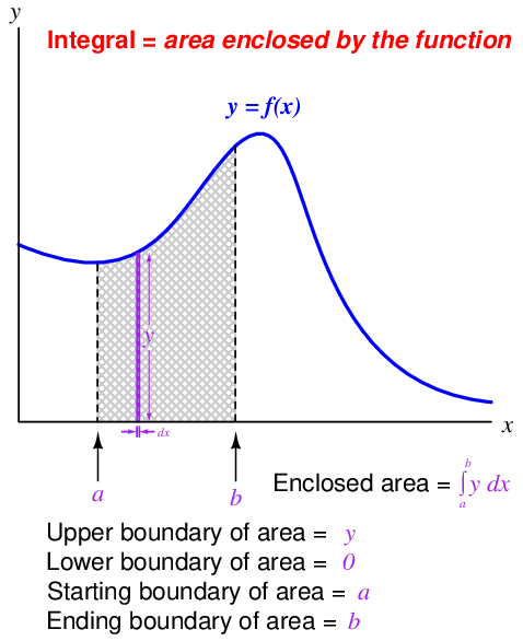
Next, let us review some of the properties of integrals, referencing the expression and graph shown below:
- An integral is always a sum of products: a process of multiplication (to calculate the product of two variables) followed by addition (to sum those quantities into a whole).
- The units of measurement for an integral reflect this initial process of multiplication: one unit times some other unit (e.g. kilowatt-hours, foot-pounds, volt-seconds).
- When computing the value of an integral, we must specify both the starting and ending points along the function defining the interval of integration (a and b).
- Geometrically, the integral of a function is the graphical area enclosed by the function and the interval boundaries.
- The area enclosed by the function may be thought of as an infinite sum of extremely narrow rectangles, each rectangle having a height equal to one variable (y) and a width equal to the differential of another variable (dx).
Just as division and multiplication are inverse mathematical functions (i.e. one “un-does” the other), differentiation and integration are also inverse mathematical functions. The two examples of propane gas flow and mass measurement highlighted in the previous sections illustrates this complementary relationship. We may use differentiation with respect to time to convert a mass measurement (m) into a mass flow measurement (W, or dm/dt ). Conversely, we may use integration with respect to time to convert a mass flow measurement (W, or dm/dt ) into a measurement of mass gained or lost (Δm).
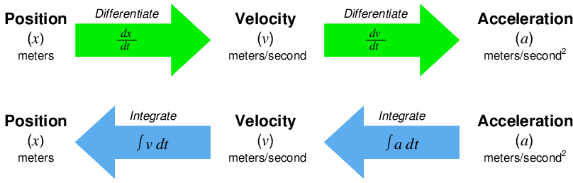
Likewise, the common examples of position (x), velocity (v), and acceleration (a) used to illustrate the principle of differentiation are also related to one another by the process of integration. Reviewing the derivative relationships:


Now, expressing position and velocity as integrals of velocity and acceleration, respectively9 :


Differentiation and integration may be thought of as processes transforming these quantities into one another. Note the transformation of units with each operation – differentiation always divides while integration always multiplies:
The inverse nature of these two calculus operations is codified in mathematics as the Fundamental Theorem of Calculus, shown here:
![[ ]
-d- ∫ b
dx a f(x)dx = f(x)](https://www.technocrazed.com/books/Instrumentation/Book_half44x.png)
What this equation tells us is that the derivative of the integral of any continuous function is that original function. In other words, we can take any mathematical function of a variable that we know to be continuous over a certain range – shown here as f(x), with the range of integration starting at a and ending at b – integrate that function over that range, then take the derivative of that result and end up with the original function. By analogy, we can take the square-root of any quantity, then square the result and end up with the original quantity, because these are inverse functions as well.
A feature of this book which may be helpful to your understanding of derivatives, integrals, and their relation to each other is found in an Appendix section . In this section, a series of illustrations provides a simple form of animation you may “flip” through to view the filling and emptying of a water storage tank, with graphs showing stored volume (V ) and volumetric flow rate (Q). Since flow rate is the time-derivative of volume (Q = dV /dt ) and volume change is the time-integral of volumetric flow rate (ΔV = ∫ Q dt), the animation demonstrates both concepts in action.