
As we have seen, the concept of differentiation is finding the rate-of-change of one variable compared to another (related) variable. In this section, we will explore the practical application of this concept to real-world data, where actual numerical values of variables are used to calculate relative rates of change.
In industrial instrumentation, for example, we are often interested in knowing the rate of change of some process variable (pressure, level, temperature, flow, etc.) over time, and so we may use computers to calculate those rates of change, either after the fact (from recorded data) or in real time (as the data is being received by sensors and acquired by the computer). We may be similarly interested in calculating the rate at which one process variable changes with respect to another process variable, both of which measured and recorded as tables of data by instruments.
Numerical (data-based) differentiation is fundamentally a two-step arithmetic process. First, we must use subtraction to calculate the change in a variable between two different points. Actually, we perform this step twice to determine the change in two variables which we will later compare. Then, we must use division to calculate the ratio of the two variables’ changes, one to the other (i.e. the “rise-over-run” steepness of the function’s graph).
For example, let us consider the application of pressure measurement for a pipeline. One of the diagnostic indicators of a burst pipeline is that the measured pressure rapidly drops. It is not the existence of low pressure in and of itself that suggests a breach, but rather the rate at which the pressure falls that reveals a burst pipe. For this reason, pipeline control systems may be equipped with automatic shut-down systems triggered by rate-of-change pressure calculations.
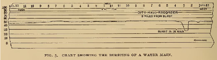
The association of rapid pressure drop with pipeline ruptures is nothing new to pipeline operations. Here is an illustration taken from page 566 of volume 8 of Cassier’s Magazine published in the year 1895, showing water pressure measurements taken by a paper strip chart recorder on a city water main line. The pressure drop created by a burst in that 36-inch pipe is clearly seen and commented on the recording:
An example of a modern11 pressure-trend recording during a pipeline rupture is shown here:
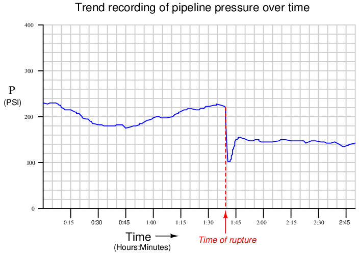
While it may seem surprising that pipeline pressure should recover after the low point immediately following the pipe’s rupture, it is important to bear in mind that many pipelines are pressure-controlled processes. After a pipeline ruptures, the pumping equipment will attempt to compensate for the reduced pressure automatically, which is why the pressure jumps back up (although not to its previous level) after the initial drop.
This phenomenon helps explain why pressure rate-of-change is a more reliable diagnostic indicator of a ruptured pipe than pressure magnitude alone: any automatic rupture-detection scheme based on a simple comparison of pipeline pressure against a pre-set threshold may fail to reliably detect a rupture if the pressure-regulating equipment is able to quickly restore pipeline pressure following the rupture. A rate-of-change system, on the other hand, will still detect the rupture based on the sharp pressure decrease following the break, even if the pressure quickly recovers.
A computer tasked with calculating the pressure’s rate of change over time (dP/dt ) would have to continuously sample the pressure value over short time periods, then calculate the quotient of pressure changes over time changes. Given a sample rate of once every 5 minutes, we see how the computer would tabulate the pressure data over time:
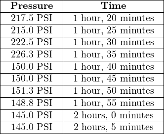
To calculate the rate of pressure change over time in each of these periods, the computer would subtract the two adjacent pressure values, subtract the two corresponding adjacent time values, and then divide those two differences to arrive at a figure in units of PSI per minute. Taking the first two data coordinates in the table as an example:

The sample period where the computer would detect the pipeline rupture lies between 1:35 and 1:40. Calculating this rate of pressure change:

Clearly, a pressure drop rate of −15.26 PSI per minute is far greater than a typical drop of −0.5 PSI per minute, thus signaling a pipeline rupture.
As you can see, the pipeline monitoring computer is not technically calculating derivatives (dP/dt ), but rather difference quotients (ΔP/Δt ). Being a digital device, the best it can ever do is perform calculations at discrete points in real time. It is evident that calculating rates of change over 5-minute period misses a lot of detail12 . The actual rate of change at the steepest point of the pressure drop far exceeds −15.26 PSI per minute.
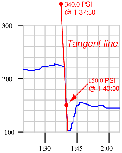
It is possible for us to calculate the instantaneous rate-of-change of pressure (dP/dt ) at the moment of the rupture by examining the graph and sketching a straight line called a tangent line matching the slope where the graph is steepest. Our goal is to calculate the exact slope of that single (steepest) point on that graph, rather than an estimate of slope between two points as the computer did. In essence, the computer “drew” short line segments between pairs of points and calculated the slopes (rise-over-run) of those line segments. The slope of each line segment13 is a difference quotient: ΔP Δt . The slope of a tangent line matching the slope at a single point on the function graph, however, is a derivative: dP/dt .
First we sketch a tangent line (by hand) matching the steepest portion of the pressure trend graph. Then, we calculate the slope of a tangent line by marking convenient points14 where the line intersects major division marks on the graph’s graduated scale, then calculating rise over run:

This distinction between calculating difference quotients (ΔP/Δt ) and calculating true derivative values (dP/dt ) becomes less and less significant as the calculation period shortens. If the computer could sample and calculate at infinite speed, it would generate true derivative values instead of approximate derivative values.
An algorithm applicable to calculating rates of change in a digital computer is shown here, using a notation called pseudocode15 . Each line of text in this listing represents a command for the digital computer to follow, one by one, in order from top to bottom. The LOOP and ENDLOOP markers represent the boundaries of a program loop, where the same set of encapsulated commands are executed over and over again in cyclic fashion:
Pseudocode listing
language=pseudocode LOOP SET x = analog˙input˙N // Update x with the latest measured input SET t = system˙time // Sample the system clock
SET delta˙x = x – last˙x // Calculate change in x SET delta˙t = t – last˙t // Calculate change in t (time)
SET rate = (delta˙x / delta˙t) // Calculate ratio of changes
SET last˙x = x // Update last˙x value for next program cycle SET last˙t = t // Update last˙t value for next program cycle ENDLOOP
Each SET command tells the computer to assign a numerical value to the variable on the left-hand side of the equals sign (=), according to the value of the variable or expression on the right-hand side of the equals sign. Text following the double-dash marks (//) are comments, included only to help human readers interpret the code, not for the computer’s benefit.
This computer program uses two variables to “remember” the values of the input (x) and time (t) from the previous scan, named last_x and last_t, respectively. These values are subtracted from the current values for x and t to yield differences (delta_x and delta_t, respectively), which are subsequently divided to yield a difference quotient. This quotient (rate) may be sampled in some other portion of the computer’s program to trigger an alarm, a shutdown action, or simply display and/or record the rate value for a human operator’s benefit.
The time period (Δt) for this program’s difference quotient calculation is simply how often this algorithm “loops,” or repeats itself. For a modern digital microprocessor, this could be many thousands of times per second.
If a nearly-instantaneous calculation is required for a rate-of-change variable, we may turn to an older technology using analog electronic circuitry. Such a differentiator circuit uses the natural behavior of a capacitor to generate an output voltage proportional to the instantaneous rate-of-change of the input voltage:
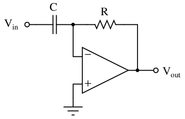
The negative feedback of the operational amplifier forms a virtual ground at the node where the capacitor, resistor, and inverting input connect. This means the capacitor “sees” the full input voltage (V in) at all times. Current through a capacitor is a direct function of the voltage’s time-derivative:

This current finds its way through the feedback resistor, developing a voltage drop that becomes the output signal (V out). Thus, the output voltage of this analog differentiator circuit is directly proportional to the time-derivative of the input voltage (i.e. the input voltage’s rate-of-change).
It is indeed impressive that such a simple circuit, possessing far fewer components than a microprocessor, is actually able to do a better job at calculating the real-time derivative of a changing signal than modern digital technology. The only real limitations to this device are accuracy (tolerances of the components used) and the bandwidth of the operational amplifier.
It would be a mistake, though, to think that an analog differentiator circuit is better suited to industrial applications of rate calculation than a digital computer, even if it does a superior job differentiating live signals. A very good argument for favoring difference quotients over actual derivatives is the presence of noise in the measured signal. A true differentiator, calculating the actual time-derivative of a live signal, will pick up on any rise or fall of the signal over time, no matter how brief. This is a serious problem when differentiating real-world signals, because noise (small amounts of “jittering” in the signal caused by any number of phenomena) will be interpreted by a perfect differentiator as very large rates of change over time.
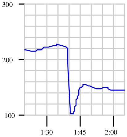
A close look at the previous pipeline pressure trend illustrates this problem. Note the areas circled (in red) on the graph, representing relatively small increases and decreases in signal occurring over very short periods of time:

Although each “step” in pressure at these circled locations is small in amplitude, each one occurs over an extremely brief time increment. Thus, each of these steps has a nearly infinite rate of change (i.e. a vertical slope). Any rate-of-change sensing system able to apply true differentiation to the pressure signal would falsely declare an alarm (high rate-of-change) condition every time it encountered one of these “steps” in the signal. This means that even under perfectly normal operating conditions the rate-detection system would periodically declare an alarm (or perhaps shut the pipeline down!) given the inevitable presence of small noise-induced16 “jitters” in the signal.
The best solution to this problem is to use a digital computer to calculate rates of change, setting the calculation period time slow enough that these small “jitters” will be averaged to very low values, yet fast enough that any serious pressure rate-of-change will be detected if it occurs. Back in the days when analog electronic circuits were the only practical option for calculating rates of signal change, the solution to this problem was to place a low-pass filter before the differentiator circuit to block such noise from ever reaching the differentiator.
Differentiation with respect to time has many applications, but there are other applications of differentiation in industrial measurement and control that are not time-based. For example, we may use differentiation to express the sensitivity of a non-linear device in terms of the rate-of-change of output over input.
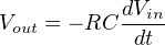
One such application is the sensitivity of a mechanism called a baffle/nozzle assembly used in many pneumatic instruments to convert a small physical motion (x) into an air pressure signal (P). This very simple mechanism uses a flat piece of sheet metal (the baffle) to restrict air flow out of a small nozzle, causing a variable “backpressure” at the nozzle to develop as the baffle-to-nozzle clearance changes:
The graph expressing the relationship between P and x is clearly non-linear, having different slopes (dP/dx ) at different points along its range. When used as part of the feedback mechanism for a self-balancing instrument, the purpose of the baffle/nozzle assembly is to detect baffle motion as sensitively as possible: that is, to generate the greatest change in pressure (ΔP) for the least change in motion (Δx). This means the designer of the pneumatic instrument should design it in such a way that the normal baffle/nozzle clearance gap rests at a point of maximum slope (maximum dP/dx ) on the graph.
Sketching a tangent line near the point of maximum slope (maximum “steepness” on the graph) allows us to approximate the rate of change at that point:
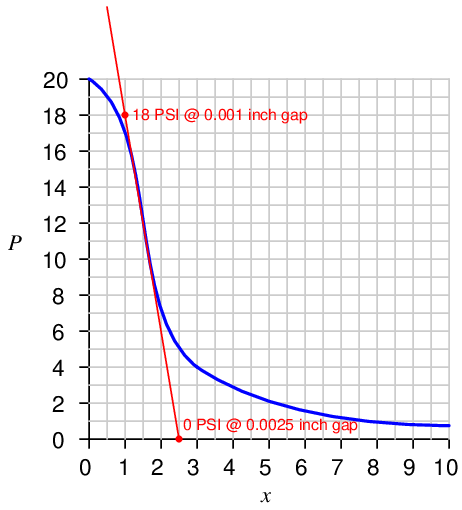
Choosing convenient points17 on this tangent line aligning with major divisions on the graph’s scales, we find two coordinates we may use to calculate the derivative of the curve at its steepest point:

The phenomenally large value of −12000 PSI per inch is a rate of pressure change to clearance (baffle-nozzle gap) change. Do not mistakenly think that this value suggests the mechanism could ever develop a pressure of 12000 PSI – it is simply describing the extreme sensitivity of the mechanism in terms of PSI change per unit change of baffle motion. By analogy, just because an automobile travels at a speed of 70 miles per hour does not mean it must travel 70 miles in distance!
It should be clear from an examination of the graph that this high sensitivity extends approximately between the pressure values of 9 and 14 PSI. Outside of those pressure values, the graph’s slope begins to decrease. While still sensitive, the baffle/nozzle mechanism will not be as sensitive to baffle motion outside those pressure values as it is within.