
In this section I will show screenshots from a process loop simulation program illustrating the effectiveness of Ziegler-Nichols open-loop (“Reaction Rate”) and closed-loop (“Ultimate”) PID tuning methods, and then contrast them against the results of my own heuristic tuning. As you will see in some of these cases, the results obtained by either Ziegler-Nichols method tends toward instability (excessive oscillation of the process variable following a setpoint change). This is not necessarily an indictment of Ziegler’s and Nichols’ recommendations as much as it is a demonstration of the power of understanding. Ziegler and Nichols presented a simple step-by-step procedure for obtaining approximate PID tuning constant values based on closed-loop and open-loop process responses, which could be applied by anyone regardless of their level of understanding PID control theory. If I were tasked with drafting a procedure to instruct anyone to quantitatively determine PID constant values without an understanding of process dynamics or process control theory, I doubt my effort would be an improvement. Ultimately, robust PID control is attainable only at the hands of someone who understands how PID works, what each mode does (and why), and is able to distinguish between intrinsic process characteristics and instrument limitations. The purpose of this section is to clearly demonstrate the limitations of ignorantly-followed procedures, and contrast this “mindless” approach against the results of simple experimentation directed by qualitative understanding.
Each of the examples illustrated in this section were simulations run on a computer program called PC-ControLab developed by Wade Associates, Inc. Although these are simulated processes, in general I have found similar results using both Ziegler-Nichols and heuristic tuning methods on real processes. The control criteria I used for heuristic tuning were fast response to setpoint changes, with minimal overshoot or oscillation.
30.5.1 Tuning a “generic” process
Ziegler-Nichols open-loop tuning procedure
The first process tuned in simulation was a “generic” process, unspecific in its nature or application. Performing an open-loop test (two 10% output step-changes made in manual mode, both increasing) on this process resulted in the following behavior:

From the trend, we can see that this process is self-regulating, with multiple lags and some dead time. The reaction rate (R) is 20% over 15 minutes, or 1.333 percent per minute. Dead time (L) appears to be approximately 2 minutes. Following the Ziegler-Nichols recommendations for PID tuning based on these process characteristics (also including the 10% step-change magnitude Δm):
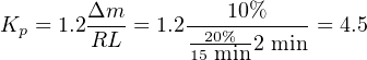


Applying the PID values of 4.5 (gain), 4 minutes per repeat (integral), and 1 minute (derivative) gave the following result in automatic mode (with a 10% setpoint change):
The result is reasonably good behavior with the PID values predicted by the Ziegler-Nichols open-loop equations, and would be acceptable for applications where some setpoint overshoot were tolerable.
We may tell from analyzing the phase shift between the PV and OUT waveforms that the dominant control action here is proportional: each negative peak of the PV lines up fairly close with each positive peak of the OUT, for this reverse-acting controller. If we were interested in minimizing overshoot and oscillation, the logical choice would be to reduce the gain value somewhat.
Ziegler-Nichols closed-loop tuning procedure
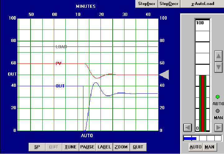
Next, the closed-loop, or “Ultimate” tuning method of Ziegler and Nichols was applied to this process. Eliminating both integral and derivative control actions from the controller, and experimenting with different gain (proportional) values until self-sustaining oscillations of consistent amplitude38 were obtained, gave a gain value of 11:
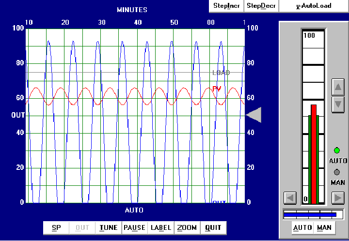
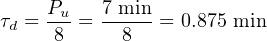
From the trend, we can see that the ultimate period (Pu) is approximately 7 minutes in length. Following the Ziegler-Nichols recommendations for PID tuning based on these process characteristics:

It should be immediately apparent that these tuning parameters will yield poor control. While the integral and derivative values are close to those predicted by the open-loop (Reaction Rate) method, the gain value calculated here is even larger than what was calculated before. Since we know proportional action was excessive in the last tuning attempt, and this one recommends an even higher gain value, we can expect our next trial to oscillate even worse.
Applying the PID values of 6.6 (gain), 3.5 minutes per repeat (integral), and 0.875 minute (derivative) gave the following result in automatic mode:

This time the loop stability is a bit worse than with the PID values given by the Ziegler-Nichols open-loop tuning equations, owing mostly to the increased controller gain value of 6.6 (versus 4.5). Proportional action is still the dominant mode of control here, as revealed by the minimal phase shift between PV and OUT waveforms (ignoring the 180 degrees of shift inherent to the controller’s reverse action).
In all fairness to the Ziegler-Nichols technique, the excessive controller gain value probably resulted more from the saturated output waveform than anything else. This led to more controller gain being necessary to sustain oscillations, leading to an inflated Kp value.
Heuristic tuning procedure
From the initial open-loop (manual output step-change) test, we could see this process contains multiple lags in addition to about 2 minutes of dead time. Both of these factors tend to limit the amount of gain we can use in the controller before the process oscillates. Both Ziegler-Nichols tuning attempts confirmed this fact, which led me to try much lower gain values in my initial heuristic tests. Given the self-regulating nature of the process, I knew the controller needed integral action, but once again the aggressiveness of this action would be necessarily limited by the lag and dead times. Derivative action, however, would prove to be useful in its ability to help “cancel” lags, so I suspected my tuning would consist of relatively tame proportional and integral values, with a relatively aggressive derivative value.
After some experimenting, the values I arrived at were 1.5 (gain), 10 minutes (integral), and 5 minutes (derivative). These tuning values represent a proportional action only one-third as aggressive as the least-aggressive Ziegler-Nichols recommendation, an integral action less than half as aggressive as the Ziegler-Nichols recommendations, and a derivative action five times more aggressive than the most aggressive Ziegler-Nichols recommendation. The results of these tuning values in automatic mode are shown here:
With this PID tuning, the process responded with much less overshoot of setpoint than with the results of either Ziegler-Nichols technique.
30.5.2 Tuning a liquid level process
Ziegler-Nichols open-loop tuning procedure
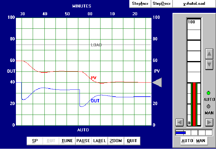
The next simulated process I attempted to tune was a liquid level-control process. Performing an open-loop test (one 10% increasing output step-change, followed by a 10% decreasing output step-change, both made in manual mode) on this process resulted in the following behavior:

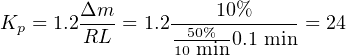
From the trend, the process appears to be purely integrating, as though the control valve were throttling the flow of liquid into a vessel with a constant out-flow. The reaction rate (R) on the first step-change is 50% over 10 minutes, or 5 percent per minute. Dead time (L) appears virtually nonexistent, estimated to be 0.1 minutes simply for the sake of having a dead-time value to use in the Ziegler-Nichols equations. Following the Ziegler-Nichols recommendations for PID tuning based on these process characteristics (also including the 10% step-change magnitude Δm):


Applying the PID values of 24 (gain), 0.2 minutes per repeat (integral), and 0.05 minutes (derivative) gave the following result in automatic mode:
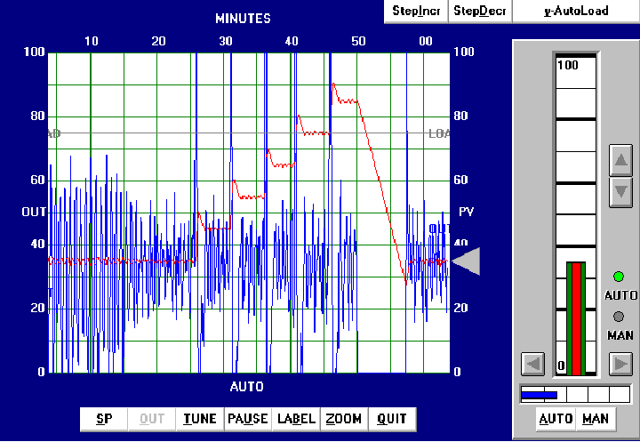
The process variable certainly responds rapidly to the five increasing setpoint changes and also to the one large decreasing setpoint change, but the valve action is hopelessly chaotic. Not only would this “jittery” valve motion prematurely wear out the stem packing, but it would also result in vast over-consumption of compressed air to continually stroke the valve from one extreme to the other. Furthermore, we see evidence of “overshoot” at every setpoint change, most likely from excessive integral action.
We can see from the valve’s wild behavior even during periods when the process variable is holding at setpoint that the problem is not a loop oscillation, but rather the effects of process noise on the controller. The extremely high gain value of 24 is amplifying PV noise by that factor, and reproducing it on the output signal.
Ziegler-Nichols closed-loop tuning procedure
Next, I attempted to perform a closed-loop “Ultimate” gain test on this process, but I was not successful. Even the controller’s maximum possible gain value would not generate oscillations, due to the extremely crisp response of the process (minimal lag and dead times) and its integrating nature (constant phase shift of −90o).
Heuristic tuning procedure
From the initial open-loop (manual output step-change) test, we could see this process was purely integrating. This told me it could be controlled primarily by proportional action, with very little integral action required, and no derivative action whatsoever. The presence of some process noise is the only factor limiting the aggressiveness of proportional action. With this in mind, I experimented with increasingly aggressive gain values until I reached a point where I felt the output signal noise was at a maximum acceptable limit for the control valve. Then, I experimented with integral action to ensure reasonable elimination of offset.
After some experimenting, the values I arrived at were 3 (gain), 10 minutes (integral), and 0 minutes (derivative). These tuning values represent a proportional action only one-eighth as aggressive as the Ziegler-Nichols recommendation, and an integral action fifty times less aggressive than the Ziegler-Nichols recommendation. The results of these tuning values in automatic mode are shown here:

You can see on this trend five 10% increasing setpoint value changes, with crisp response every time, followed by a single 50% decreasing setpoint step-change. In all cases, the process response clearly meets the criteria of rapid attainment of new setpoint values and no overshoot or oscillation.
If it was decided that the noise in the output signal was too detrimental for the valve, we would have the option of further reducing the gain value and (possibly) compensating for slow offset recovery with more aggressive integral action. We could also attempt the insertion of a damping constant into either the level transmitter or the controller itself, so long as this added lag did not cause oscillation problems in the loop39 . The best solution would be to find a way to isolate the level transmitter from noise, so that the process variable signal was much “quieter.” Whether or not this is possible depends on the process and on the particular transmitter used.
30.5.3 Tuning a temperature process
Ziegler-Nichols open-loop tuning procedure
This next simulated process is a temperature control process. Performing an open-loop test (two 10% increasing output step-changes, both made in manual mode) on this process resulted in the following behavior:
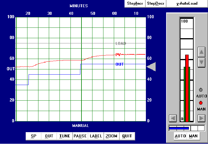
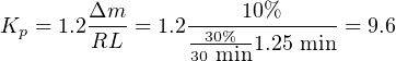
From the trend, the process appears to be self-regulating with a slow time constant (lag) and a substantial dead time. The reaction rate (R) on the first step-change is 30% over 30 minutes, or 1 percent per minute. Dead time (L) looks to be approximately 1.25 minutes. Following the Ziegler-Nichols recommendations for PID tuning based on these process characteristics (also including the 10% step-change magnitude Δm):


Applying the PID values of 9.6 (gain), 2.5 minutes per repeat (integral), and 0.625 minutes (derivative) gave the following result in automatic mode:

As you can see, the results are quite poor. The PV is still oscillating with a peak-to-peak amplitude of almost 20% from the last process upset at the time of the 10% downward SP change. Additionally, the output trend is rather noisy, indicating excessive amplification of process noise by the controller.
Ziegler-Nichols closed-loop tuning procedure
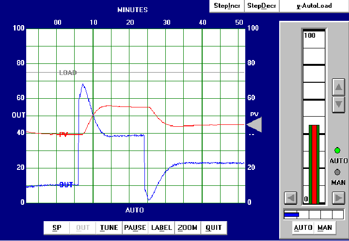
Next, the closed-loop, or “Ultimate” tuning method of Ziegler and Nichols was applied to this process. Eliminating both integral and derivative control actions from the controller, and experimenting with different gain (proportional) values until self-sustaining oscillations of consistent amplitude were obtained, gave a gain value of 15:
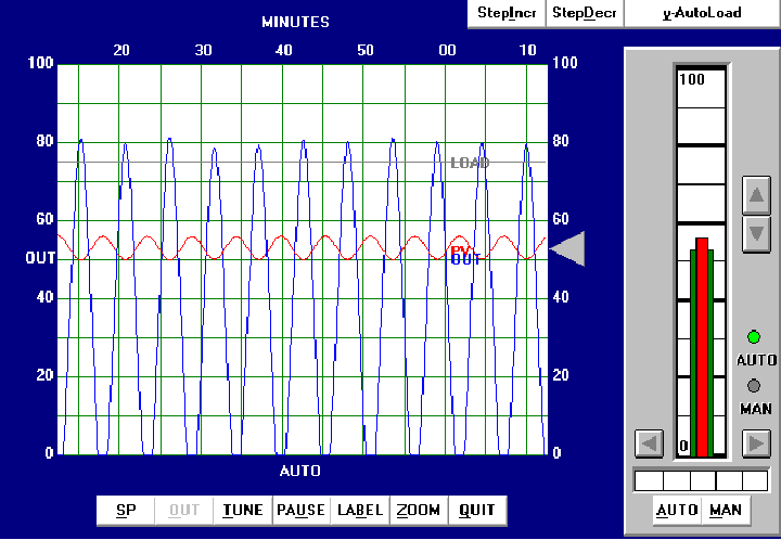
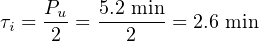
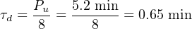
From the trend, we can see that the ultimate period (Pu) is approximately 5.2 minutes in length. Following the Ziegler-Nichols recommendations for PID tuning based on these process characteristics:

These PID tuning values are quite similar to those predicted by the open loop (“Reaction Rate”) method, and so we would expect to see very similar results:

As expected, we still see excessive oscillation following a 10% setpoint change, as well as excessive “noise” in the output trend.
Heuristic tuning procedure
From the initial open-loop (manual output step-change) test, we could see this process was self-regulating with a slow lag and substantial dead time. The self-regulating nature of the process demands at least some integral control action to eliminate offset, but too much will cause oscillation given the long lag and dead times. The existence of over 1 minute of process dead time also prohibits the use of aggressive proportional action. Derivative action, which is generally useful in overcoming lag times, will cause problems here by amplifying process noise. In summary, then, we would expect to use mild proportional, integral, and derivative tuning values in order to achieve good control with this process. Anything too aggressive will cause problems for this process.
After some experimenting, the values I arrived at were 3 (gain), 5 minutes (integral), and 0.5 minutes (derivative). These tuning values represent a proportional action only one-third as aggressive as the Ziegler-Nichols recommendation, and an integral action about half as aggressive as the Ziegler-Nichols recommendation. The results of these tuning values in automatic mode are shown here:
As you can see, the system’s response has almost no overshoot (with either a 10% setpoint change or a 15% setpoint change) and very little “noise” on the output trend. Response to setpoint changes is relatively crisp considering the naturally slow nature of the process: each new setpoint is achieved within about 7.5 minutes of the step-change.