30.4 Heuristic PID Tuning Procedures

In contrast to quantitative tuning procedures where definite numerical values for P, I, and D controller settings are obtained through data collection and analysis, a heuristic tuning procedure is one where general rules are followed to obtain approximate or qualitative results. The majority of PID loops in the world have been tuned with such methods, for better or for worse. My goal in this section is to optimize the effectiveness of such tuning methods.

When I was first educated on the subject of PID tuning, I learned this rather questionable tuning procedure:

Configure the controller for proportional action only (integral and derivative control actions set to minimum effect), setting the gain near or at 1.
Increase controller gain until self-sustaining oscillations are achieved, “bumping” the setpoint value up or down as necessary to provoke oscillations.
When the ultimate gain is determined, reduce the aggressiveness of proportional action by a factor of two.
Repeat steps 2 and 3, this time adjusting integral action instead of proportional.
Repeat steps 2 and 3, this time adjusting derivative action instead of proportional.

The first three steps of this procedure are identical to the steps recommended by Ziegler and Nichols for closed-loop tuning. The last two steps are someone else’s contribution. The results of this method are generally poor, and I strongly recommend against using it!

While this particular procedure is crude and ineffective, it does illustrate a useful principle in trial-and-error PID tuning: we can tune a PID-controlled process by incrementally adjusting the aggressiveness of a controller’s P, I, and/or D actions until we see oscillations (suggesting the action has become too aggressive), then reducing the aggressiveness of the action until stable control is achieved. The “trick” to doing this effectively and efficiently is knowing which action(s) to focus on, which action(s) to avoid, and how to tell which of the actions is too aggressive when things do begin to oscillate. The following portions of this subsection describe the utility of each control action, the limitations of each, and how to recognize an overly-aggressive condition.

Much improvement may be made to any “trial-and-terror” PID tuning procedure if one is aware of the process characteristics and recognizes the applicability of P, I, and D actions to those process characteristics. Random experimentation with P, I, and D parameter values is tedious at best and dangerous at worst! As always, the key is to understand the role of each action, their applicability to different process types, and their limitations. The competent loop-tuner should be able to visually analyze trends of PV, SP, and Output, and be able to discern the degrees of P, I, and D action in effect at any given time in that trend.

Here is an improved PID tuning technique employing heuristics (general rules) regarding P, I, and D actions. It is assumed that you have taken all necessary safety precautions (e.g. you know the hazards of the process and the limits you are allowed to change it) and other steps recommended in the “Before You Tune . . .” section (30.2) beginning on page 4029:

Perform open-loop (manual-mode) tests of the process to determine its natural characteristics (e.g. self-regulating versus integrating versus runaway, steady-state gain, noisy versus calm, dead time, time constant, lag order) and to ensure no field instrument or process problems exist (e.g. control valve with excessive friction, inconsistent process gain, large dead time). Correct all problems before proceeding³² .
Identify any controller actions that may be problematic (e.g. derivative action on a noisy process), noting to use them sparingly or not at all.
Identify whether the process will depend mostly on proportional action or integral action for stability. This will be the controller’s “dominant” action when tuned. You may find the chart on page 4057 useful for this.
Start with all terms of the controller set for minimal response (minimal P, minimal I, no D).
Set the dominant action to some safe value³³ (e.g. gain less than 1, integral time much longer than time constant of process) and check the loop’s response to setpoint and/or load changes in automatic mode.
Increase aggressiveness of this action until a point is reached where any more causes excessive overshoot or oscillation.
Increase aggressiveness of the other action(s) as needed to achieve the best compromise between stability and quick response.
If the loop ever shows signs of being too aggressive (e.g. oscillations), use the technique of phase-shift comparison between PV and Output trends (see page 4059) to identify which controller action to attenuate.
Repeat the last three steps as often as needed.

Note: the loop should never “porpoise” (see page 4066) when responding to a setpoint or load change! Some oscillation around setpoint may be tolerable (especially when optimizing the tuning for fast response to setpoint and load changes), but “porpoising” is always something to avoid.

30.4.1 Features of P, I, and D actions

Purpose of each action

Proportional action is the “universal” control action, capable of providing at least marginal control quality for any process.
Integral action is useful for eliminating offset caused by load variations and process self-regulation.
Derivative action is useful for canceling lags, but useless by itself.

Limitations of each action

Proportional action will cause oscillations if sufficiently aggressive, in the presence of lags and/or dead time. The more lags (higher-order), the worse the problem. It also directly reproduces process noise onto the output signal.
Integral action will cause oscillation if sufficiently aggressive, in the presence of lags and/or dead time. Any amount of integral action will guarantee overshoot following setpoint changes in purely integrating processes.
Derivative action dramatically amplifies process noise, and will cause oscillations in fast-acting processes.

Special applicability of each action

Proportional action works exceptionally well when aggressively applied to processes lacking the phase shift necessary to oscillate: self-regulating processes dominated by first-order lag, and purely integrating processes.
Integral action works exceptionally well when aggressively applied to fast-acting, self-regulating processes. Has the unique ability to ignore process noise.
Derivative action works exceptionally well to speed up the response of processes dominated by large lag times, and to help stabilize runaway processes. Small amounts of derivative action will sometimes allow more aggressive P and/or I actions to be used than otherwise would be possible without unacceptable overshoot.

Gain and phase shift of each action

Proportional action acts on the present, adding no phase shift to a sinusoidal signal. Its gain is constant for any signal frequency.
Integral action acts on the past, adding a −90^o phase shift to a sinusoidal signal. Its gain decreases with increasing frequency.
Derivative action acts on the future, adding a +90^o phase shift to a sinusoidal signal. Its gain increases with increasing frequency.

30.4.2 Tuning recommendations based on process dynamics

Knowing which control actions to focus on first is a matter of characterizing the process (identifying whether it is self-regulating, integrating, runaway, noisy, has lag or dead time, or any combination of these traits based on an open-loop response test³⁴ ) and then selecting the best actions to fit those characteristics. The following table shows some general recommendations for fitting PID tuning to different process characteristics

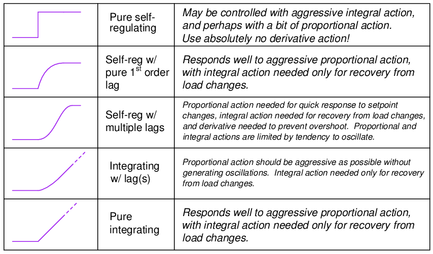
General rules:

Use no derivative action if the process signal is “noisy”
Use proportional action sparingly if the process signal is “noisy”
The slower the time lag(s), the less integral action to use (a good approximation is to set the integration time τ_i equal to the measured lag time of the process)
The higher-order the time lag(s), the less proportional action (gain) to use
Self-regulating processes need integral action
Integrating processes need proportional action
Dead time requires a reduction of all PID constants below what would normally work

Once you have determined the basic character of the process, and understand from that characterization what the needs of the process will be regarding P, I, and/or D control actions, you may “experiment” with different tuning values of P, I, and D until you find a combination yielding robust control.

30.4.3 Recognizing an over-tuned controller by phase shift

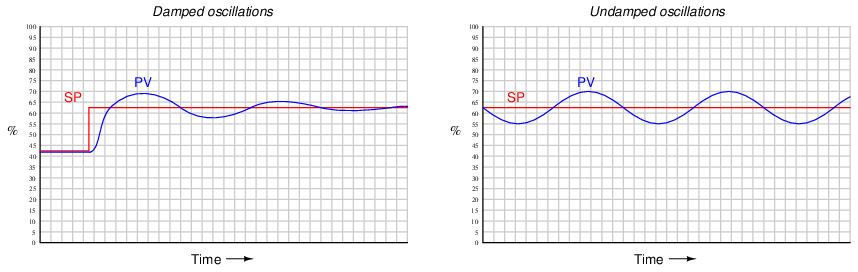
When performing heuristic tuning of a PID controller, it is important to be able to identify a condition where one or more of the “actions” (P, I, or D) is configured too aggressively for the process. The characteristic indication of over-tuning is the presence of sinusoidal oscillations. At best, this means damped oscillations following a sudden setpoint or load change. At worst, this means oscillations that never decay:

At this point, the question is: which action of the controller is causing this oscillation? We know all three actions (P, I, and D) are fully capable of causing process oscillation if set too aggressive, so in the lack of clarifying information it could be any of them (or some combination!).

One clue is the trend of the controller’s output compared with the trend of the process variable (PV). Modern digital control systems all have the ability to trend manipulated variables as well as process variables, allowing personnel to monitor exactly how a loop controller is managing a process. If we compare the two trends, we may examine the phase shift between PV and output of a loop controller to discern what it’s dominant action is.

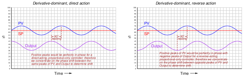
For example, the following trend graphs show the PV and output signals for a loop controller with proportional-dominant response. Both direct- and reverse-acting versions are shown:

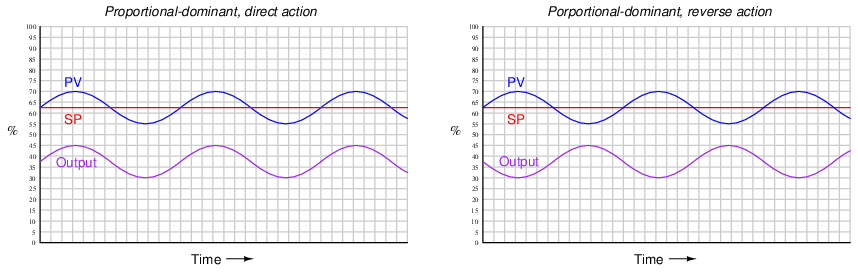
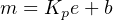
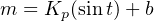
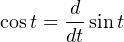
Since we know proportional action is immediate, there should be no phase shift³⁵ between the PV and output waveforms. This makes sense from a mathematical perspective: if we substitute a sine function for the error variable in a proportional-only controller equation, we see that different gain values (K_p) simply result in an output signal of the same phase, just amplified or attenuated:

If ever you see a process oscillating like this (sinusoidal waveforms, with the PV and output signals in-phase), you know that the controller’s response to the process is dominated by proportional action, and that the gain needs to be reduced (i.e. increase proportional band) to achieve stability.

Integral and derivative actions, however, introduce phase shift between the PV waveform and the output waveform. The direction of phase shift will reveal which time-based action (either I or D) dominates the controller’s response and is therefore most likely the cause of oscillation.

For example, the following trend graph shows the PV and output signals for a loop controller with integral-dominant response. Both direct- and reverse-acting versions are shown:

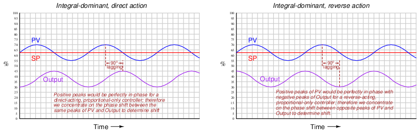
Here, the output waveform is phase-shifted 90^o behind (lagging) the PV waveform compared to what it would be by proportional action alone. This −90^o phase shift is most difficult to see for reverse-acting controllers, since the natural 180^o phase shift caused by reverse action makes the additional −90^o shift look like a +90^o shift (i.e. a −270^o shift). One method I use for discerning the direction of phase shift for reverse acting controllers is to imagine what the output waveform would look like for a proportional-only controller, and compare to that. Another method is to perform a “thought experiment” looking at the PV waveform, noting the velocity of the controller’s output at points of maximum error (when integral action would be expected to move the output signal fastest). In the previous example of an integral-dominant reverse-acting controller, we see that the output signal is indeed descending at its most rapid pace when the PV is highest above setpoint (greatest positive error), which is exactly what we would expect reverse-acting integration to do.

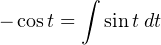
Mathematically, this makes sense as well. Integration of a sine function results in a negative cosine waveform:

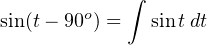
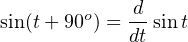
Another way of stating this is to say integration always adds a −90^o phase shift:

If derivative action is set too aggressive for the needs of the process, the resulting output waveform will be phase-shifted +90^o from that of a purely proportional response:

Once again, the direction of phase shift is easiest to discern in the direct-acting case, since we expect the PV and output sine waves to be perfectly in-phase for proportional-dominant response. A +90^o phase shift is very clear to see in the direct-acting example because the peaks of the output waveform clearly precede the corresponding peaks of the PV waveform. The reverse-acting control example is more difficult due to the added 180^o of phase shift intrinsic to reverse action.

The derivative of a sine function is always a cosine function (or alternatively stated, a sine function with a +90^o phase shift):

You may encounter cases where multiple PID terms are set too aggressively for the needs of the process, in which case the phase shift will be split somewhere between 0^o and ± 90^o owing to the combined actions. In such cases one must “round up” or “round down” the phase shift to the nearest value of −90⁰, 0^o, or +90^o in order to determine which of the three actions (I, P, or D, respectively) is most responsible for the oscillations.

30.4.4 Recognizing a “porpoising” controller

An interesting case of over-tuning is when the process variable “porpoises³⁶ ” on its way to setpoint following a step-change in setpoint. The following trend shows such a response:

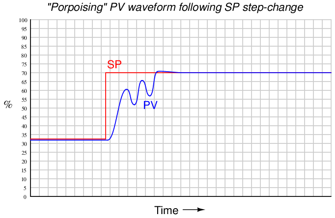
“Porpoising” is universally poor behavior for a loop, because it combines the negative consequences of over-tuning (instability and excessive valve travel) with the negative consequence of under-tuning (delay achieving setpoint). There is no practical purpose served by a loop “porpoising,” and so this behavior should be avoided if at all possible.

Thankfully, identifying the cause of “porpoising” is rather easy to do. Only two control actions are capable of causing this response: proportional and derivative. Integral action simply cannot cause porpoising. In order for the process variable to “porpoise,” the controller’s output signal must reverse direction before the process variable ever reaches setpoint. Integral action, however, will always drive the output in a consistent direction when the process variable is on one side of setpoint. Only proportional and derivative actions are capable of producing a directional change in the output signal prior to reaching setpoint.

Solely examining the process variable waveform will not reveal whether it is proportional action, derivative action, or both responsible for the “porpoising” behavior. A trial reduction in the derivative³⁷ tuning parameter is one way to identify the culprit, as is phase-shift analysis between the PV and output waveforms during the “porpoising” period.

Back to Main Index of Book