
Control valves are subject to a number of common problems. This section is dedicated to an exploration of the more common control valve problems, and potential remedies.
27.14.1 Mechanical friction
Control valves are mechanical devices with moving parts, and as such they are subject to friction, primarily between the valve stem and the stem packing. Some degree of friction is inevitable in valve packing49 and in some types of trim where components must move past each other throughout the full range of valve stem travel (e.g. cage-guided globe valves, rotary ball valves) the trim itself adds additional friction beyond that which is imposed by the packing.
In physics, friction is classified as either static or dynamic. Static friction is defined as frictional force holding two stationary objects together. Dynamic friction is defined as frictional force impeding the motion of two objects sliding past each other. Static friction is always greater in magnitude than dynamic friction. Anyone who has ever pulled a sled through snow or ice knows that more force is required to “break” the sled loose from a stand-still (static friction) than is required to keep it moving (dynamic friction). The same holds true for friction in a control valve: the amount of force required to initially overcome static friction (i.e. initiate valve stem motion) usually exceeds the amount of force required to maintain the valve stem in motion.
The presence of friction in a control valve increases the force necessary from the actuator to cause valve movement. If the actuator is electric or hydraulic, the only real problem with increased force is the additional energy required from the actuator to move the valve (recall that mechanical work is the product of force and parallel displacement). If the actuator is pneumatic, however, a more serious problem arises from the combined effects of static and dynamic friction.
A simple “thought experiment” illustrates the problem. Imagine an air-to-open, sliding-stem control valve with the lower bench-set pressure applied to the pneumatic actuator. This should be the amount of pressure where the valve is just about to open from a fully-closed position. Now imagine slowly increasing the air pressure applied to the actuator. What should this valve do? If the spring tension is set properly, and there is negligible friction in the valve, the stem should smoothly rise from the fully-closed position as pressure increases beyond the bench-set pressure. However, what will this valve do if there is substantial friction present in the valve assembly? Instead of the stem smoothly lifting immediately as pressure exceeds the bench-set value, this valve will remain fully closed until enough extra pressure has accumulated in the actuator to generate a force large enough to overcome spring tension plus valve friction. Then, once the stem “breaks free” from static friction and begins to move, the stem will begin to accelerate because the actuator force now exceeds the sum of spring tension and friction, since dynamic friction is less than static friction. Compressed air trapped inside the actuator acts like a spring of its own, releasing stored energy. As the stem moves, however, the chamber volume in the diaphragm or piston actuator increases, causing pressure to drop, which causes the actuating force to decrease. When the force decreases sufficiently, the stem stops moving and static friction “grabs” it again. The stem will remain stationary until the applied pressure increases sufficiently again to overcome static friction, then the “slip-stick” cycle repeats.
If we graph the mechanical response of a pneumatic actuator with substantial stem friction, we see something like this:
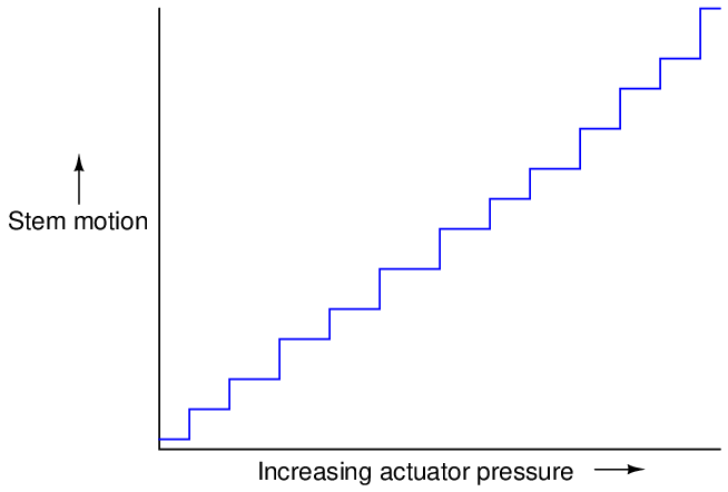
What should be a straight, smooth line is reduced to a series of “stair-steps” as the combined effect of static and dynamic friction, plus the dynamic effects of a pneumatic actuator, conspire to make precise stem positioning nearly impossible. This effect is commonly referred to as stiction.
Even worse is the effect friction has on valve position when we reverse the direction of pressure change. Suppose that after we have reached some new valve position in the opening direction, we begin to ramp the pneumatic pressure downward. Due to static friction (again), the valve will not immediately respond by moving in the closed direction. Instead, it will hold still until enough pressure has been released to diminish actuator force to the point where there is enough unbalanced spring force to overcome static friction in the downward direction. Once this static friction is overcome, the stem will begin to accelerate downward because (lesser) dynamic friction will have replaced (greater) static friction. As the stem moves, however, air volume inside the actuating diaphragm or piston chamber will decrease, causing the contained air pressure to rise. Once this pressure rises enough that the stem stops moving downward, static friction will again “grab” the stem and hold it still until enough of a pressure change is applied to the actuator to overcome static friction.
What may not be immediately apparent in this second “thought experiment” is the amount of pressure change required to cause a reversal in stem motion compared to the amount of pressure change required to provoke continued stem motion in the same direction. In order to reverse the direction of stem motion, not only does the static friction have to be “relaxed” from the last movement, but additional static friction must be overcome in the opposite direction before the stem is able to move that way. We may clarify this concept by applying the problem-solving strategy of adding numerical quantities to the thought experiment. Suppose we have a control valve with a static packing friction of 50 pounds in either direction, and a diaphragm with a 12-inch diameter (113.1 square inches of area). According to the force/pressure/area formula (F = PA), an applied pressure of 0.442 PSI will be required to overcome this static friction in either direction. That is to say, when moving in the upward direction, we must apply 0.442 PSI more pressure than is ideally required to achieve any given valve position. If after achieving this stem position we desire to move the valve downward to some new stem position, we must not only decrease the pressure by 0.442 PSI to relax the tension on the packing, but we must also decrease it another 0.442 PSI to overcome packing friction in the downward direction before the valve moves at all from its last position. Thus, a pressure reversal of 0.884 PSI (i.e. twice the equivalent value of packing friction) is required to make the valve reverse its direction of motion. This constitutes “deadband” in the control valve’s action, which degrades control behavior.
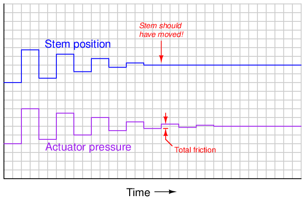
Thus, the effects of friction on a pneumatic control valve actuator may be quantified by subjecting the valve to small reversals in applied actuator pressure and measuring the resulting stem position. The largest increment of actuator pressure reversal resulting in zero stem motion represents the total amount of friction within the valve mechanism.
The following graph shows such a test, plotting actuator pressure over time as well as valve stem position over time. As the actuator pressure is stepped up and down in successively smaller intervals, the control valve’s stem position is seen to respond with less and less motion until it fails to respond at all:
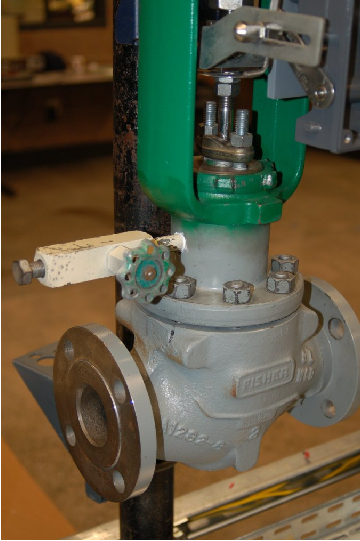
Short of rebuilding a “sticky” control valve to replace damaged or worn components, there is not much that may be done to improve valve stiction other than regular lubrication of the packing (if appropriate). Lubrication is applied to the packing by means of a special lubricator device threaded into the bonnet of the valve:
As one of the common sources of excessive packing friction is over-tightening of the packing nuts by maintenance personnel eager to prevent process fluid leaks, a great deal of trouble may be avoided simply by educating the maintenance staff on the “care and feeding” of control valve packing for long service life.
Many modern digital valve positioners have the ability to monitor the drive force applied by an actuator on a valve stem, and correlate that force against stem motion. Consequently, it is possible to perform highly informative diagnostic tests on a control valve’s mechanical “health,” at least with regard to friction50 . For pneumatic and hydraulic actuators, actuator force is a simple and direct function of fluid pressure applied to the piston or diaphragm. For electric actuators, actuator force is an indirect function of electric motor current, or may be directly measured using load cells or springs and displacement sensors in the gear mechanism.
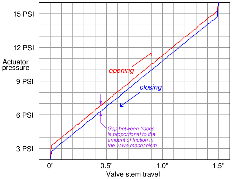
The following valve signature illustrates the kind of diagnostic “audit” that may be obtained from a digital control valve positioner based on actuator force (pneumatic air pressure) and stem motion:
This same diagnostic tool is useful for detecting trim seating problems in valve designs where there is sliding contact between the throttling element and the seat near the position of full closure (e.g. gate valves, ball valves, butterfly valves, plug valves, etc.). The force required to “seat” the valve into the fully-closed position will naturally be greater than the force required to move the throttling element during the rest of its travel, but this additional force should be smooth and consistent on the graph. A “jagged” force/travel graph near the fully-closed position indicates interference between the moving element and the stationary seat, providing information valuable for predicting the remaining service life of the valve before the next rebuild.
27.14.2 Flashing
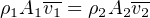
When a fluid passes through the constrictive passageways of a control valve, its average velocity increases. This is predicted by the Law of Continuity, which states that the product of fluid density (ρ), cross-sectional area of flow (A), and average velocity (v) must remain constant for any flowstream:
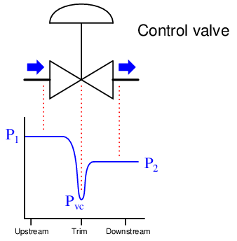
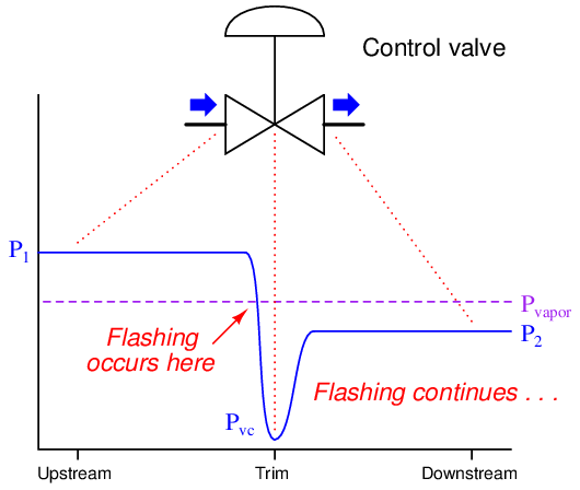
As fluid velocity increases through the constrictive passages of a control valve, the fluid molecules’ kinetic energy increases. In accordance with the Law of Energy Conservation, potential energy in the form of fluid pressure must decrease correspondingly. Thus, fluid pressure decreases within the constriction of a control valve’s trim as it throttles the flow, then increases (recovers) after leaving the constrictive passageways of the trim and entering the wider areas of the valve body:

If the fluid being throttled by the valve is a liquid (as opposed to a gas or vapor), and its absolute pressure ever falls below the vapor pressure51 of that substance, the liquid will begin to boil. This phenomenon, when it happens inside a control valve, is called flashing. As the graph shows, the point of lowest pressure inside the valve (called the vena contracta pressure, or Pvc) is the location where flashing will first occur, if it occurs at all.
Flashing is almost universally undesirable in control valves. The effect of boiling liquid at the point of maximum constriction is that flow through the valve becomes “choked” by the rapid expansion of liquid to vapor as it boils, degrading the valve’s flow capacity (i.e. decreasing the effective Cv). Flashing is also destructive to the valve trim, as boiling action propels tiny droplets of liquid at extremely high velocities past the plug and seat faces, eroding the metal over time.
A photograph showing a severely eroded valve plug (from a cage-guided globe valve) reveals just how destructive flashing can be:
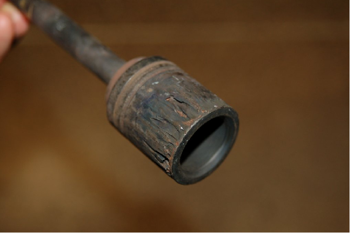
A characteristic effect of flashing in a control valve is a “hissing” sound, reminiscent of what sand might sound like if it were flowing through the valve.
An important parameter predicting flashing in a control valve is the valve’s pressure recovery factor, based on a comparison of the valve’s total pressure drop from inlet to outlet versus the pressure drop from inlet to the point of minimum pressure within the valve.
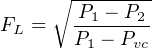
Where,
FL = Pressure recovery factor (unitless)
P1 = Absolute fluid pressure upstream of the valve
P2 = Absolute fluid pressure downstream of the valve
Pvc = Absolute fluid pressure at the vena contracta (point of minimum fluid pressure within the valve)
The following set of illustrations shows three different control valves exhibiting the same permanent pressure drop (P1 − P2), but having different values of FL:
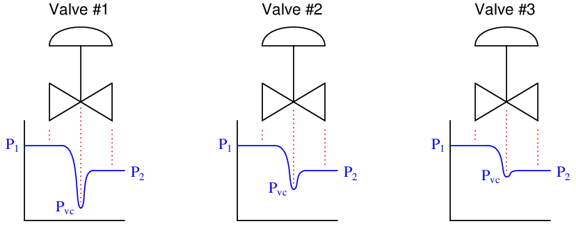
Valve #1 exhibits the greatest pressure recovery (i.e. the amount that fluid pressure increases from the minimum pressure at the vena contracta to the downstream pressure: P2 − Pvc) and the lowest FL value. It is also the valve most prone to flashing in liquid service, because the vena contracta pressure is so much lower (all other factors being equal) than in the other two valves. If any of these valves will experience flashing in liquid service, it would be valve #1.
Valve #3, by contrast, has very little pressure recovery, and a large FL value (nearly equal to 1). From the perspective of avoiding flashing, it is the best of the three valves to use for liquid service.
The style of valve (ball, butterfly, globe, etc.) is very influential on pressure recovery factor. The more convoluted the path for fluid within a control valve, the more opportunities that fluid will have to dissipate energy in turbulent motion, resulting in the greatest permanent pressure drop for the least amount of restriction at any single point in the flow’s path.
Compare these two styles of valve to see which will have lowest pressure recovery factor and therefore be most prone to flashing:
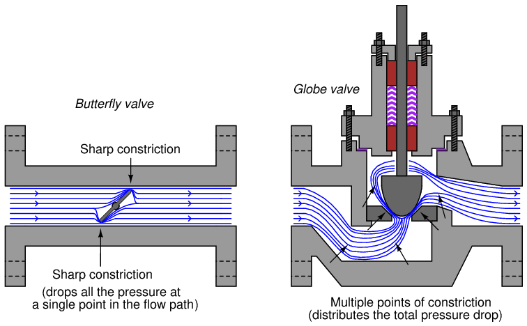
Clearly, the globe valve does a better job of evenly distributing pressure losses throughout the path of flow. By contrast, the butterfly valve can only drop pressure at the points of constriction between the disk and the valve body, because the rest of the valve body is a straight-through path for fluid offering little restriction at all. As a consequence, the butterfly valve experiences a much lower vena contracta pressure (i.e. greater pressure recovery, and a lower FL value) than the globe valve for any given amount of permanent pressure loss, making the butterfly valve more prone to flashing than the globe valve with all other factors being equal.
27.14.3 Cavitation
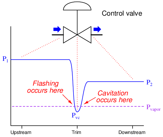
Fluid passing through a control valve experiences changes in velocity as it enters the narrow constriction of the valve trim (increasing velocity) then enters the widening area of the valve body downstream of the trim (decreasing velocity). These changes in velocity result in the fluid molecules’ kinetic energies changing as well, in accordance with the kinetic energy equation Ek = 1 2mv2. In order that energy be conserved in a moving fluid stream, any increase in kinetic energy due to increased velocity must be accompanied by a complementary decrease in potential energy, usually in the form of fluid pressure. This means the fluid’s pressure will fall at the point of maximum constriction in the valve (the vena contracta, at the point where the trim throttles the flow) and rise again (or recover) downstream of the trim:
If fluid being throttled is a liquid, and the pressure at the vena contracta is less than the vapor pressure of that liquid at the flowing temperature, the liquid will spontaneously boil. This is the phenomenon of flashing previously described. If, however, the pressure recovers to a point greater than the vapor pressure of the liquid, the vapor will re-condense back into liquid again. This is called cavitation.
As destructive as flashing is to a control valve, cavitation is worse. When vapor bubbles re-condense into liquid they often do so asymmetrically, one side of the bubble collapsing before the rest of the bubble. This has the effect of translating the kinetic energy of the bubble’s collapse into a high-speed “jet” of liquid in the direction of the asymmetrical collapse. These liquid “microjets” have been experimentally measured at speeds up to 100 meters per second (over 320 feet per second). What is more, the pressure applied to the surface of control valve components in the path of these microjets is intense. Each microjet strikes the valve component surface over a very small surface area, resulting in a very high pressure (P = F A) applied to that small area. Pressure estimates as high as 1500 newtons per square millimeter (1.5 giga-pascals, or about 220000 PSI!) have been calculated for cavitating control valve applications involving water.
No substance known is able to continuously withstand this form of abuse, meaning that cavitation will destroy any control valve given enough time. The effect of each microjet impinging on a metal surface is to carve out a small pocket in that metal surface. Over time, the metal will begin to take on a “pock-marked” look over the area where cavitation occurs. This stands in stark contrast to the visual appearance of flashing damage, which is smooth and polished.
Photographs of a fluted valve plug and its matching seat are shown here as evidence of flashing and cavitation damage, respectively:
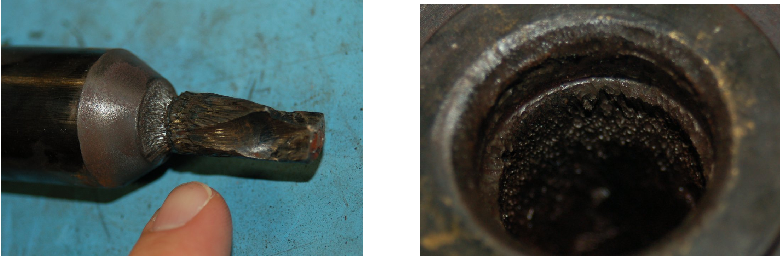
The plug of this valve has been severely worn by flashing and cavitation. The flashing damage is responsible for the relatively smooth wear areas seen on the plug. Cavitation damage is most prominent inside the seat, where almost all the damage is in the form of pitting. The mouth of the seat exhibits smooth wear caused by flashing, but deeper inside you can see the pock-marked surface characteristic of cavitation, where liquid microjets literally blasted away pieces of metal. This trim set belongs to a Fisher Micro-Flat Cavitation valve, designed with process liquid flow passing down instead of up (i.e. first past the wide body of the plug and then down through the seat, rather than first up through the seat and then past the wide body of the plug). This trim design does not prevent cavitation (as clearly evidenced by the photos), but it does “move” the area of cavitation damage down below the seat’s sealing surface into a long tube extending below the seat. Although the ravages of flashing clearly took their toll on this valve’s trim, the valve would have been rendered inoperable much sooner had cavitation been at work along the plug’s length and at the sealing area where the plug contacts the seat.
The sound made by substantial liquid cavitation also contrasts starkly against the sound made by flashing. Whereas flashing sounds as though sand were flowing through the valve, cavitation produces a much louder “crackling” sound comprised of distinct impact pulses, reminiscent of what gravel or rocks might sound like if they were somehow forced to flow through the valve.
Sustained cavitation also has the detrimental effect of accelerating corrosion in certain process services. Bare metal surfaces are highly reactive with many chemical fluids, but become more resistant to further attack when a thin layer of reacted metal on the surface (the so-called passivation layer) acts as a sort of chemical barrier. Rust on steel, or the powdery-white oxide of aluminum are good examples: the initially bare metal surfaces react with their surrounding environment to form a protective outer layer, impeding further degradation of the metal beneath that layer. Cavitation works to blast away any protective layer that might otherwise accumulate, allowing corrosion to work at full speed until the entire thickness of the metal is corroded through. The complementary destructive actions of cavitation and corrosion together is sometimes referred to as cavitation corrosion.
Several methods exist for abating cavitation in control valves:
- Prevent flashing in the first place
- Cushion with introduced gas
- Sustain the flashing action (i.e. delay cavitation)
Cavitation abatement method #1 is quite simple to understand: if we prevent flashing from ever happening in a control valve, cavitation cannot follow. The key to doing this is making sure the vena contracta pressure never falls below the vapor pressure for the liquid. Several techniques exist for doing this:
- Select a control valve type having less pressure recovery (i.e. greater FL value)
- Increase both upstream and downstream pressures by relocating the valve to a higher-pressure location in the process.
- Use multiple control valves in series to reduce the lowest pressure at either one
- Decrease the liquid’s temperature (this decreases vapor pressure)
- Use cavitation-control valve trim
The last suggestion in this list deserves further exploration. Valve trim may be specially designed for cavitation abatement by providing multiple stages of pressure drop for the fluid as it passes through the trim. The following is a pressure versus location graph for a cavitating control valve. The liquid’s vapor pressure is shown here as a dashed line marked Pvapor:
A valve equipped with cavitation-control trim will have a different pressure profile, with multiple vena contracta points where the fluid passes through a series of constrictions within the trim itself:
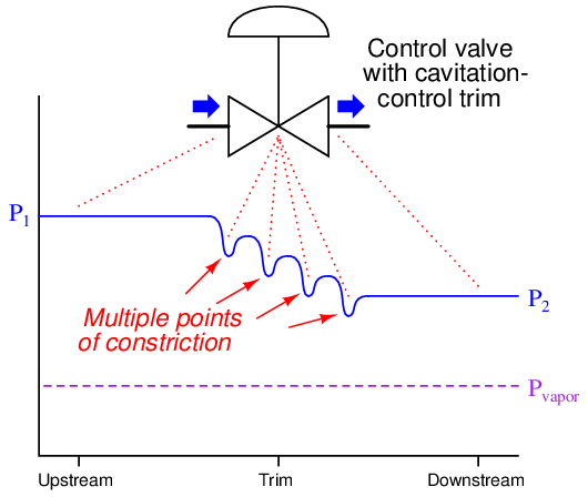
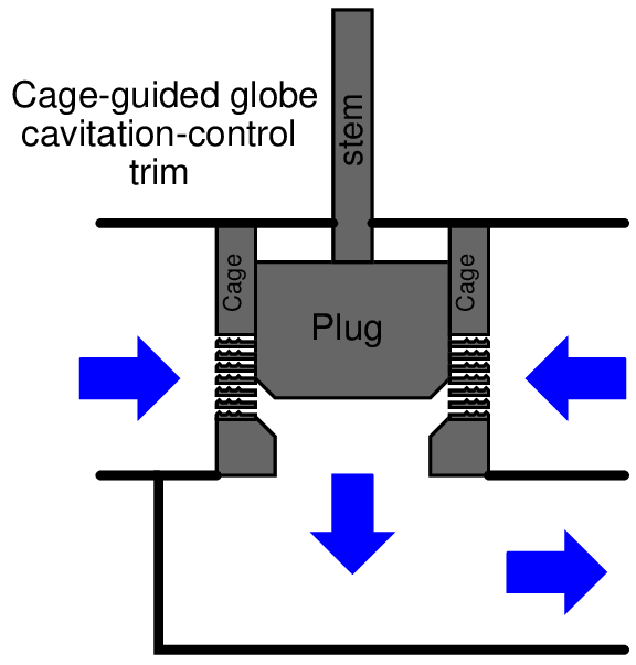
This way, the same final permanent pressure drop (P1 − P2) may be achieved without the lowest pressure ever falling below the liquid’s vapor pressure limit. An example of cavitation-control design applied to cage-guided globe valve trim is shown in the following illustration:
Ball-style control valves, with their relatively high pressure recovery (low pressure recovery factor FL values) are more prone to cavitation than globe valves, all other factors being equal. Special ball trim designed to help distribute pressure drops over a longer flow path is available, an example of this shown in the next photograph:
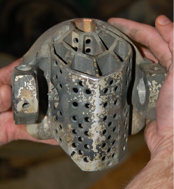
The round (ball-shaped) portion of the trim is on the far side of this piece, with the cavitation-controlling structure visible in the foreground. Fluid flow passing through the gap between the ball’s edge and the valve seat spills into this multi-chambered structure where turbulence helps develop pressure drops at several locations. In a normal ball valve, there is only one location for any substantial pressure drop to develop, and that is at the narrow gap between the ball’s edge and the seat. Here, multiple regions of pressure drop exist, with the intent of avoiding the liquid’s vapor pressure limit at any one location, thus eliminating flashing and consequently eliminating cavitation.
Cavitation abatement method #2 is practical only in some process applications, where a non-reacting gas may be injected into the liquid stream to provide some “cushioning” within the cavitating region. The presence of non-condensible gas bubbles in the liquid stream disturbs the microjets’ pathways, helping to dissipate their energy before striking the valve body walls.
Cavitation abatement method #3 involves a strategy opposite that of method #1. If, for whatever reason, we cannot avoid falling below the vapor pressure of the liquid as the flow stream moves through the valve, we may have the option of ensuring the downstream liquid pressure never rises above the liquid’s vapor pressure, at least until the fluid clears past the valuable control valve and into an area of the system where cavitation damage will not be so expensive. This avoids cavitation at the cost of guaranteed flashing within the control valve, which is generally not as destructive as cavitation.
A pressure diagram shows how this method works:
Of course, flashing is not good for a control valve either. Not only does it damage the valve over time, but it also causes problems with flow capacity, as we will explore next.
27.14.4 Choked flow
Both gas and liquid control valves may experience what is generally known as choked flow. Simply put, “choked flow” is a condition where the rate of flow through a valve does not change substantially as downstream pressure is reduced.
Ideally, turbulent fluid flow rate through a control valve is a simple function of valve flow capacity (Cv) and differential pressure drop (P1 − P2), as described by the basic valve flow equation:
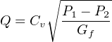
This equation simply does not apply for choked-flow conditions.
In a gas control valve, choking occurs when the velocity of the gas reaches the speed of sound for that gas. This is often referred to as critical or sonic flow. In a liquid control valve, choking occurs with the onset of flashing52 . The reason sonic velocity is relevant to flow capacity for a control valve has to do with the propagation of pressure changes in fluids. Pascal’s principle tells us that changes in pressure within a closed fluid system will manifest at all points in the fluid system, but this never happens instantaneously. Instead, pressure changes propagate through any fluid at the speed of sound within that fluid. If a fluid stream happens to move at or above the speed of sound, pressure changes downstream are simply not able to overcome the stream’s velocity to affect anything upstream, which explains why the flow rate through a control valve experiencing sonic (critical) flow velocities does not change with changes in downstream pressure: those downstream pressure changes cannot propagate upstream against the fast-moving flow, and so will have no effect on the flow as it accelerates to sonic velocity at the point(s) of constriction.

Choked flow conditions become readily apparent if the flow-versus-pressure function of a control valve at any fixed opening value is graphed. The basic valve flow equation predicts a perfectly straight line at constant slope with flow rate (Q) as the vertical variable and the square root of pressure drop () as the horizontal variable. However, if we actually test a control valve by holding its upstream liquid pressure (P1) constant and varying its downstream pressure (P2) while maintaining a fixed stem position, we notice a point where flow reaches a maximum limit value:
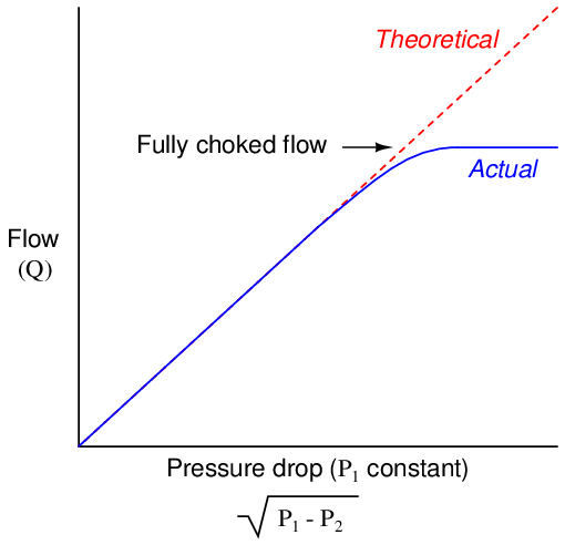
In a choked flow condition, further reductions in downstream pressure achieve no greater flow of liquid through the valve. This is not to say that the valve has reached a maximum flow – we may still increase flow rate through a choked valve by increasing its upstream pressure. We simply cannot coax any more flow through a choked valve by decreasing its downstream pressure.
An approximate predictor of choked flow conditions for gas valve service is the upstream-to-minimum absolute pressure ratio. When the vena contracta pressure is less than one-half the upstream pressure, both measured in absolute pressure units, choked flow is virtually guaranteed. One should bear in mind that this is merely an approximation and not a precise prediction for choked flow. Much more information is needed about the valve design, the particular process gas, and other factors in order to reliably predict the presence of choking.
Choked flow in liquid services is predicted when the vena contracta pressure equals the liquid’s vapor pressure, since choking is a function of flashing for liquid flowstreams.
No attempt will be made in this book to explain sizing procedures for control valves in choked-flow service, due to the complexity of the subject.
An interesting and useful application of choked flow in gases is a device called a critical velocity nozzle. This is a nozzle designed to allow a fixed flow rate of gas through it given a known upstream pressure, and a downstream pressure that is sufficiently low to ensure sonic velocities in the nozzle throat. One practical use for critical velocity nozzles is in the flow testing of compressed air systems. One or more of these nozzles are connected to the main header line of an air compressor system and allowed to vent to atmosphere. So long as the compressor(s) are able to maintain constant header pressure, the flow rate of air through the nozzles(s) is guaranteed to be fixed, allowing a technician to monitor compressor parameters under precisely known load conditions.
27.14.5 Valve noise
A troublesome phenomenon in severe services is the audible noise produced by turbulence as the fluid moves through a control valve. Noise output is worse for gas services experiencing sonic (critical) flow and for liquid services experiencing cavitation, although it is possible for a control valve to produce substantial noise even when avoiding these operating conditions. Noise produced by a control valve also translates into vibration imposed on the piping, which may cause problems such as loosening of threaded fasteners over time.
One way to reduce noise output is to use special valve trim resembling the trim used to mitigate cavitation. A common cage-guided globe valve trim design for noise reduction uses a special cage designed with numerous, small holes for process gas to flow through. One of the ways in which these small holes reduce audible noise is by shifting the frequency of that noise upward. This increase in frequency places the sound outside the range where the human ear is most sensitive to noise, and it also helps to reduce noise coupling to the piping, confining most of the noise “power” to the internal volume of the process fluid rather than radiating outward into the air.
Fisher manufactures a series of noise-abatement trim for process gas service called Whisper trim. A “Whisper” plug and cage set is shown in this next photograph:
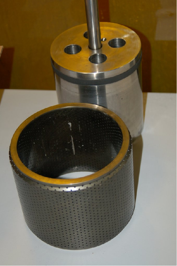
In some versions, the holes are merely straight through the cage wall. In more sophisticated versions of Whisper trim (particularly the “WhisperFlo”), the small holes lead to a labyrinth of passages designed to dissipate energy by forcing the fluid to take several sharp turns as it passes through the wall of the cage. This allows relatively large pressure drops to develop without high fluid velocities, which is the primary causal factor for noise in control valves.
27.14.6 Erosion
A problem common to control valves used in slurry service (where the process fluid is a liquid containing a substantial quantity of hard, solid particles) is erosion, where the valve trim and body are worn by the passage of solid particles. Erosion produces some of the most striking examples of valve damage, as shown by the following photographs53 :
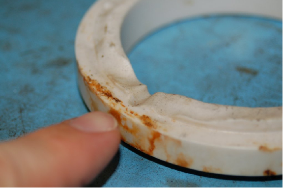
Here we see large holes worn in a globe valve plug, and substantial damage done to the seat as well. The process service in this case was water with “coke fines” (small particles of coke, a solid petroleum product). Even ceramic valve seat components are not immune to damage from slurry service, as revealed by this photograph of a valve seat with a notch worn by slurry flow:
There really is no good way to reduce the effects of erosion damage from slurry flows, other than to use exceptionally hard valve trim materials. Even then, the control valve must be considered a fast-wearing component (along with pumps and any other components in harm’s way of the slurry flowstream), rebuilt or replaced at regular intervals.
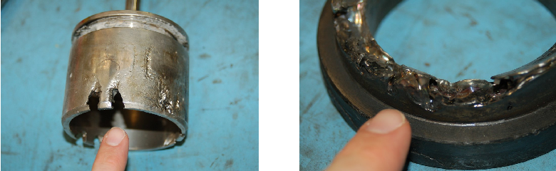
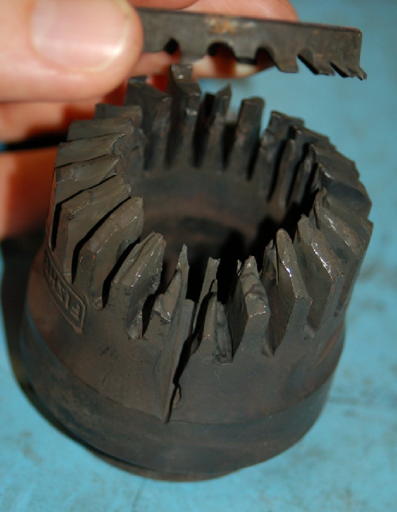
Another cause of erosion in control valves is wet steam, where steam contains droplets of liquid water propelled at high velocity by the steam flow. A dramatic example of wet steam damage appears in this next photograph, where the cage from a Fisher valve has been literally cut in half from the flow:
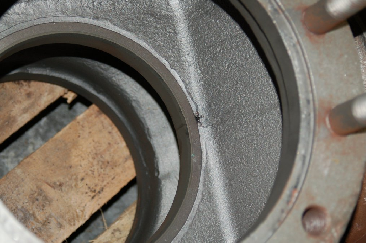
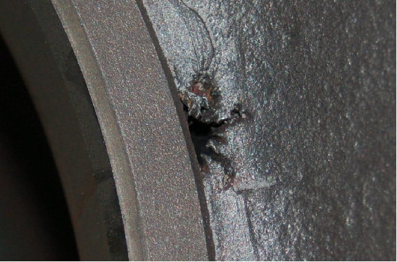
Steam may also “cut” other parts of a valve if allowed to leak past. Here, we see a valve bonnet with considerable damage caused by steam leaking past the outside of the packing, between the packing rings and the bonnet’s bore:
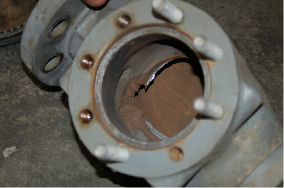
Any fluid with sufficient velocity may cause extensive damage to valve components. Small holes developing in the body of a valve may become large holes over time, as fluid rushes through the hole. The initial cause of the hole may be a manufacturing defect (such as porosity in the metal casting) or damage inflicted by the user (e.g. a crack in the valve body caused by some traumatic event). An example of such a hole in a valve body becoming worse over time appears in this next photograph, taken of a control valve removed after 40 years of continuous service:
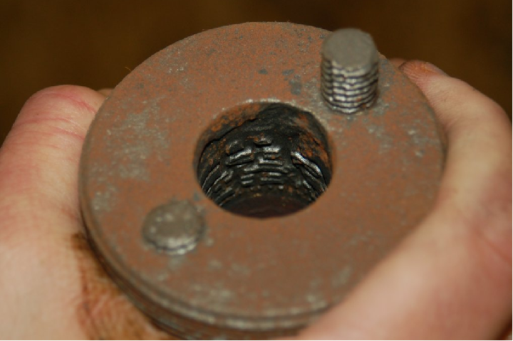
A close-up photograph of this same hole shows the leak path worn larger by passing fluid, allowing fluid to flow by the seat even with the valve in the fully-closed position:
In more severe process services, such holes rapidly grow in size. This next photograph shows a rather extreme example of a hole near the seat of a valve body, enlarged to the point where the valve is hardly capable of restricting fluid flow at all because the hole provides a bypass route for flow around the valve plug and seat:
27.14.7 Chemical attack
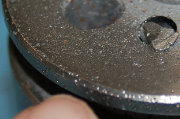
Corrosive chemicals may attack the metal components of control valves if those components are not carefully selected for the proper service. A close-up photograph of a chemically-pitted valve plug shows pitting characteristic of chemical attack:
As mentioned previously in this chapter, the effects of corrosion are multiplied when combined with the effects of cavitation. Most metals develop what is known as a passivation layer in response to chemical attack. The outer layer of metal corrodes, but the byproduct of that corrosion is a relatively inert compound acting to shield the rest of the metal from further attack. Rust on steel, or aluminum oxide on aluminum, are both common examples of passivation layers in response to oxidation of the metal. When cavitation happens inside a valve, however, the extremely high pressures caused by the liquid microjets will blast away any protection afforded by the passivation layer, allowing chemical attack to begin anew. The result is rapid degradation of the valve components.
27.15 Review of fundamental principles
Shown here is a partial listing of principles applied in the subject matter of this chapter, given for the purpose of expanding the reader’s view of this chapter’s concepts and of their general inter-relationships with concepts elsewhere in the book. Your abilities as a problem-solver and as a life-long learner will be greatly enhanced by mastering the applications of these principles to a wide variety of topics, the more varied the better.
- Definition of pressure: P = F A (pressure is the amount of force applied over a specified area by a fluid. Relevant to fluid-powered valve actuators: the amount of force developed by an actuator is proportional to the fluid pressure applied to it and the area of its piston or diaphragm.
- Pascal’s principle: changes in fluid pressure are transmitted evenly throughout an enclosed fluid volume. Relevant to fluid-powered valve actuators.
- Fluid seals: accomplished by maintaining tight contact between solid surfaces. Relevant to control valve plug and seat design, where even seating force is critical to maintaining tight shut-off. Also relevant to valve packing design.
- Conservation of energy: energy cannot be created or destroyed, only converted between different forms. Relevant to fluid velocities and pressures inside of a control valve.
- Bernoulli’s equation: z1ρg+ v12ρ 2 +P1 = z2ρg+ v22ρ 2 +P2, which is an application of the Law of Energy Conservation, stating that the sum of all forms of energy in a moving fluid stream (height, kinetic, and pressure) must remain the same. Relevant to calculations of pressure drop and pressure recovery across control valve trim.
- Conservation of mass: mass is an intrinsic property of matter, and as such cannot be created or destroyed. Relevant to the Continuity Principle for moving fluids, where the mass flow rate of a fluid entering a control valve must equal the mass flow rate exiting the valve.
- Linear equations: any function represented by a straight line on a graph may be represented symbolically by the slope-intercept formula y = mx + b. Relevant to control valve positioners and split-ranging.
- Zero shift: any shift in the offset of an instrument is fundamentally additive, being represented by the “intercept” (b) variable of the slope-intercept linear formula y = mx + b. Relevant to control valve calibration: adjusting the “zero” of a valve positioner always adds to or subtracts from the valve stem position.
- Span shift: any shift in the gain of an instrument is fundamentally multiplicative, being represented by the “slope” (m) variable of the slope-intercept linear formula y = mx + b. Relevant to control valve calibration: adjusting the “span” of a valve positioner always multiplies or divides the stem stroke (compared to signal span).
- Deadband and hysteresis: the difference in response with the independent variable increasing versus decreasing. Usually caused by friction in a mechanism. Relevant to control valve response: a control valve will not go to the same position with its command signal at some value increasing as it does at that same value decreasing, due to friction in the trim and packing.
- Inverse mathematical functions: an inverse function, when applied to the result of its counterpart function, “un-does” the operation and leaves you with the original quantity. Relevant to control valve characterization, where the inherently nonlinear response of a control valve installed in a process with variable pressure drop is made to behave more linearly by skewing the shape of the valve trim in an inverse manner.
- Negative feedback: when the output of a system is degeneratively fed back to the input of that same system, the result is decreased (overall) gain and greater stability. Relevant to control valve positioners as well as self-actuated regulators.
- Self-balancing pneumatic mechanisms: all self-balancing pneumatic instruments work on the principle of negative feedback maintaining a nearly constant baffle-nozzle gap. Force-balance mechanisms maintain this constant gap by balancing force against force with negligible motion, like a tug-of-war. Motion-balance mechanisms maintain this constant gap by balancing one motion with another motion, like two dancers moving in unison.
References
Baumann, Hans D., Control Valve Primer, A User’s Guide, Second Edition, Instrument Society of America, Research Triangle Park, NC, 1994.
Brestel, Ronald; Hutchens, Wilbur; Wood, Charles, Control Valve Packing Systems, Technical Monograph 38, Fisher Controls International Inc., Marshalltown, IA, 1992.
“Cavitation in Control Valves”, document L351 EN, Samson AG, Frankfurt, Germany.
Control Valve Handbook, Third Edition, Fisher Controls International, Inc., Marshalltown, IA, 1999.
Control Valve Sourcebook – Power & Severe Service, Fisher Controls International, Inc., Marshalltown, IA, 1988.
“Design ED, EAD, and EDR Sliding-Stem Control Valves”, Product Bulletin 51.1:ED, Fisher, Marshalltown, IA, 2006.
Grumstrup, Bruce, Considerations in the Design and Selection of Bellows Seal Equipment Valves, Technical Monograph 37, Fisher Controls International Inc., Marshalltown, IA, 1991.
Hutchison, J.W., ISA Handbook of Control Valves, Second Edition, Instrument Society of America, Research Triangle Park, NC, 1976.
Jury, Floyd D., Fundamentals of Aerodynamic Noise in Control Valves, Technical Monograph 43, Fisher Controls International Inc., Marshalltown, IA, 1999.
Lipták, Béla G. et al., Instrument Engineers’ Handbook – Process Control Volume II, Third Edition, CRC Press, Boca Raton, FL, 1999.
“Micro Trims for Globe and Angle Valve Applications”, Product Bulletin 80.4:010, Emerson Process Management, Marshalltown, IA, 2005.
“Packing Selection Guidelines for Sliding-Stem Valves”, Product Bulletin 59.1:062, Emerson Process Management, Marshalltown, IA, 2007.
“Pipeline Accident Report – Pipeline Rupture and Subsequent Fire in Bellingham, Washington June 10, 1999”, NTSB/PAR-02/02, PB2002-916502, Notation 7264A, National Transportation Safety Board, Washington DC, 2002.
Richardson, Jonathan W., Primary Seat Shutoff, Technical Monograph 47, Fisher Controls International LLC, Marshalltown, IA, 2005.
Riveland, Marc, Fundamentals of Valve Sizing for Liquids, Technical Monograph 30, Fisher Controls International Inc., Marshalltown, IA, 1985.
Schafbuch, Paul, Fundamentals of Flow Characterization, Technical Monograph 29, Fisher Controls International Inc., Marshalltown, IA, 1985.
Warnett, Chris, Using Valve Actuators as Predictive Maintenance Tools for MOVs, Rotork Controls, Inc., Rochester, NY, 2000.
“Valve Sizing Technical Bulletin”, document MS-06-84-E, revision 3, Swagelok Company, MI, 2002.