
Control valves are supposed to deliver reliable, repeatable control of process fluid flow rate over a wide range of operating conditions. As we will soon see, this is something of a challenge, as the rate of fluid flow through a control valve depends on more than just the position of its stem. This section discusses the problem of control valve behavior in real process applications, and explores the concept of characterization as a solution to the problem.
27.13.1 Inherent versus installed characteristics
When control valves are tested in a laboratory setting, they are connected to a piping system providing a nearly constant pressure difference between upstream and downstream (P1 −P2 = constant). With a fluid of constant density and a constant pressure drop across the valve, flow rate becomes directly proportional to the valve’s flow coefficient (Cv). This is clear from an examination of the basic valve capacity equation, if we replace the pressure and specific gravity terms with a single constant k:
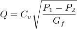


As discussed in an earlier section of this chapter (see section 27.12.1), the amount of “resistance” offered by a restriction of any kind to a turbulent fluid depends on the cross-sectional area of that restriction and also the proportion of fluid kinetic energy dissipated in turbulence. If a control valve is designed such that the combined effect of these two parameters vary linearly with stem motion, the Cv of the valve will likewise be proportional to stem position. That is to say, the Cv of a “linear” control valve will be approximately half its maximum rating with the stem position at 50%; approximately one-quarter its maximum rating with the stem position at 25%; and so on.
If such a valve is placed in a laboratory flow test piping system with constant differential pressure and constant fluid density, the relationship of flow rate to stem position will be linear. With constant pressure drop, the flow rate through any valve is directly proportional to that valve’s Cv, and with a “linear” valve design the Cv (and therefore the flow rate as well) must be directly proportional to stem position:
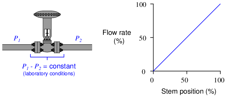
However, most real-life valve installations do not provide the control valve with a constant pressure drop. Due to frictional pressure losses in piping and changes in supply/demand pressures that vary with flow rate, a typical control valve “sees” substantial changes in differential pressure as its controlled flow rate changes. Generally speaking, the pressure drop available to the control valve decreases as flow rate increases.
The result of this pressure drop versus flow relationship is that the actual flow rate of the same valve installed in a real process will not linearly track valve stem position. Instead, it will “droop” as the valve is further opened. This “drooping” graph is called the valve’s installed characteristic, in contrast to the inherent characteristic exhibited in the laboratory with constant pressure drop:
Each time the stem lifts up a bit more to open the valve trim further, flow increases, but not as much as at lower-opening positions. It is a situation of diminishing returns, where we still see increases in flow as the stem lifts up, but to a lesser and lesser degree.
In my years of teaching, I have found this concept of “installed characteristic” to be especially challenging for many students. In the interest of clarifying the concept, the next two subsections will present a pair of contrasting valve performance scenarios.
27.13.2 Control valve performance with constant pressure
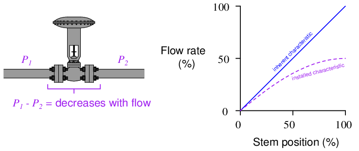
First, let us imagine a control valve installed at the base of a dam, releasing water from the reservoir. Given a constant height of water in the reservoir, the upstream (hydrostatic) pressure at the valve will likewise be constant. Let’s assume this constant upstream pressure will be 20 PSI (corresponding to approximately 46 feet of water column above the valve inlet). With the valve discharging into the air, downstream pressure will essentially be zero. This set of upstream and downstream conditions guarantees a constant pressure drop of 20 PSI across our control valve at all times, for all flow conditions:
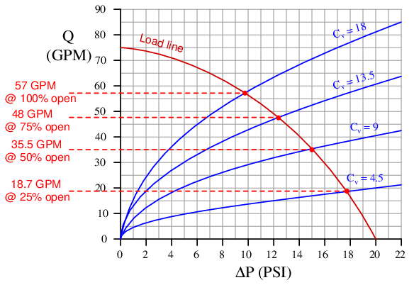
Furthermore, let us assume the control valve has a “linear” inherent characteristic and a maximum flow capacity (Cv rating) of 18. This means the valve’s Cv will be 18 at 100% open, 13.5 at 75% open, 9 at 50% open, 4.5 at 25% open, and 0 at fully closed (0% open). We may plot the behavior of this control valve at these four stem positions by graphing the amount of flow through the valve for varying degrees of pressure drop across the valve. The result is a set of characteristic curves37 for our hypothetical control valve:
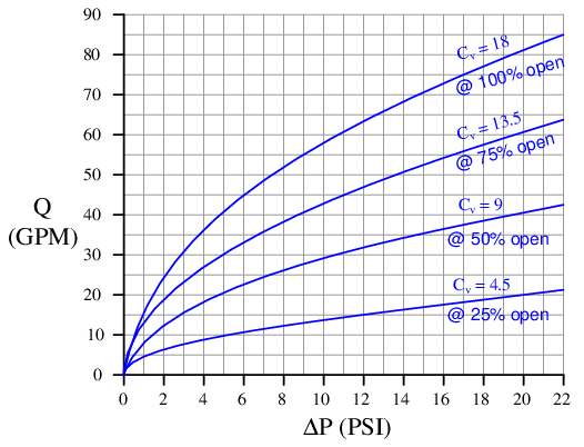

Each curve on the graph traces the amount of flow through the valve at a constant stem position, for different amounts of applied pressure drop. For example, looking at the curve representing 50% open (Cv = 9), we can see the valve should flow about 42 GPM at 22 PSI, about 35 GPM at 15 PSI, about 20 GPM at 5 PSI, and so on. Of course, we can obtain these same flow figures simply by evaluating the formula Q = Cv (which is in fact what I used to plot these curves), but the point here is to learn how to interpret the graph.
We may use this set of characteristic curves to determine how this valve will respond in any installation by superimposing another curve on the graph called a load line38 , describing the pressure drop available to the valve at different flow rates. Since we know our hypothetical dam supplies a constant 20 PSI across the control valve for all flow conditions, the load line for the dam will be a vertical line at 20 PSI:
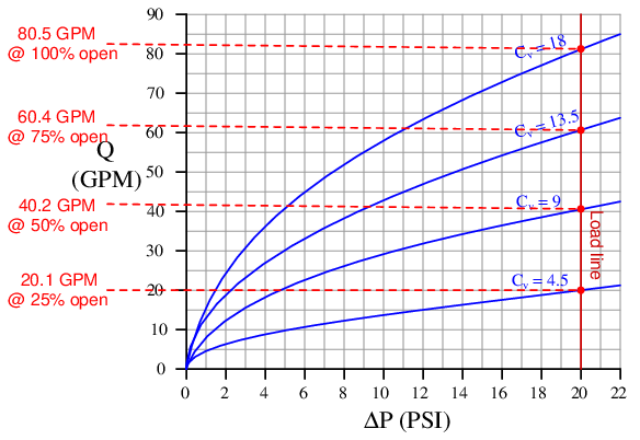
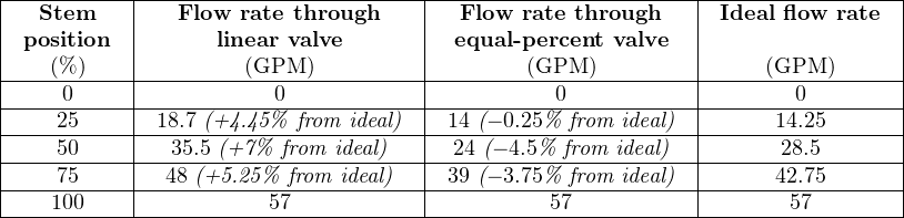
By noting the points of intersection39 between the valve’s characteristic curves and the load line, we may determine the flow rates from the dam at those stem positions:
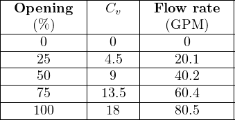
If we were to graph this table, plotting flow versus stem position, we would obtain a very linear graph. Note how 50% open gives us twice as much flow as 25% open, and 100% open nearly twice as much flow as 50% open. This tells us our control valve will respond linearly when operated under these conditions (i.e. operating with a constant pressure drop).
27.13.3 Control valve performance with varying pressure
Now let us consider a scenario where the pressure drop across the valve changes as the rate of flow through the valve changes. We may modify the previous example of a control valve releasing water from a dam to generate this effect. Suppose the valve is not closely coupled to the dam, but rather receives water through a narrow (restrictive) pipe:
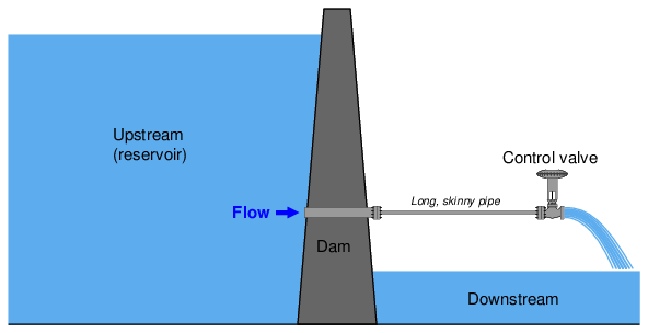
In this installation, the narrow pipe generates a flow-dependent pressure drop due to friction between the turbulent water and the pipe walls, leaving less and less upstream pressure at the valve as flow increases. The control valve still drains to atmosphere, so its downstream pressure is still a constant 0 PSIG, but now its upstream pressure diminishes with increasing flow. How will this affect the valve’s performance?
We may turn to the same set of characteristic curves to answer this question. All we need is a new load line describing the pressure available to the valve at different flow rates, then we may look for the points of intersection between this load line and the valve’s characteristic curves. For the sake of our hypothetical example, I have sketched an arbitrary “load line” (actually a load curve) showing how the valve’s pressure falls off as flow rises40 :
Now we see a definite nonlinearity in the control valve’s behavior. No longer does a doubling of stem position (from 25% to 50%, or from 50% to 100%) result in a doubling of flow rate41 :
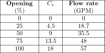
If we plot the valve’s performance in both scenarios (close-coupled to the dam, versus at the end of a restrictive pipe), we see the difference very clearly:
The “drooping” graph shows how the valve responds when it does not receive a constant pressure drop throughout the flow range. This is how the valve responds when installed in a non-ideal process, compared to the straight-line response it exhibits under ideal conditions of constant pressure. This what we mean by “installed” characteristic versus “ideal” or “inherent” characteristic.
Pressure losses due to fluid friction as it travels down pipe is just one cause of valve pressure changing with flow. Other causes exist as well, including pump curves42 and frictional losses in other system components such as filters and heat exchangers. Whatever the cause, any piping system that fails to provide constant pressure across a control valve will “distort” the valve’s inherent characteristic in the same “drooping” manner, and this must be compensated in some way if we desire linear response from the valve.
Not only does the diminishing pressure drop across the valve mean we cannot achieve the same full-open flow rate as in the laboratory (with a constant pressure drop), but it also means the control valve responds with different amounts of sensitivity at various points along its range. Note how the installed characteristic graph is relatively steep at the beginning where the valve is nearly closed, and how the graph grows “flatter” at the end where the valve is nearly full-open. The rate of response (rate-of-change of flow Q compared to stem position x, which may be expressed as the derivative dQ dx ) is much greater at low flow rates than it is at high flow rates, all due to diminished pressure drop at higher flow rates. This means the valve will respond more “sensitively” at the low end of its travel and more “sluggishly” at the high end of its travel.
From the perspective of a feedback control system, this varying valve responsiveness means the system will be unstable at low flow rates and unresponsive at high flow rates. At low flow rates – where the valve is nearly closed – any small movement of the valve stem will have a relatively large effect on fluid flow. However, at high flow rates, a much greater stem motion will be required to achieve a comparable effect on fluid flow. Thus, the control system will tend to over-react at low flow rates and under-react at high flow rates, simply because the control valve fails to exert the same degree of control over process flow at different flow rates. Oscillations may occur at low flow rates, and excessive deviations from setpoint at high flow rates as a result of this “distorted” valve behavior.
27.13.4 Characterized valve trim
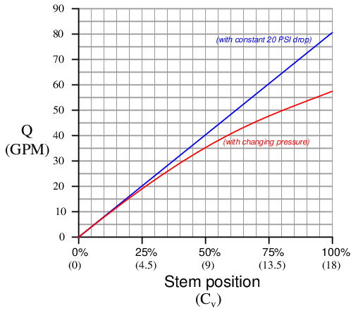
The root cause of the problem – a varying pressure drop caused by frictional losses in the piping and other factors – generally cannot be eliminated. This means there is no way to regain maximum flow capacity short of replacing the control valve with one having a greater Cv rating43 . However, there is a clever way to flatten the valve’s responsiveness to achieve a more linear characteristic, and that is to purposely design the valve such that its inherent characteristic complements the process “distortion” caused by changing pressure drop. In other words, we design the control valve trim so it opens up gradually during the initial stem travel (near the closed position), then opens up more aggressively during the final stages of stem travel (near the full-open position). With the valve made to open up in a nonlinear fashion inverse to the “droop” caused by the installed pressure changes, the two non-linearities should cancel each other and yield a more linear response.
This re-design will give the valve a nonlinear characteristic when tested in the laboratory with constant pressure drop, but the installed behavior should be more linear:
Now, control system response will be consistent at all points within the controlled flow range, which is a significant improvement over the original state of affairs.
Control valve trim is manufactured in a variety of different “characteristics” to provide the desired installed behavior. The two most common inherent characteristics are linear and equal percentage. “Linear” valve trim exhibits a fairly proportional relationship between valve stem travel and flow capacity (Cv), while “equal percentage” trim is decidedly nonlinear. A control valve with “linear” trim will exhibit consistent responsiveness only with a constant pressure drop, while “equal percentage” trim is designed to counter-act the “droop” caused by changing pressure drop when installed in a process system.
The Cv for linear and equal-percentage control valve trims are given by the following formulae44 :


Where,
Cv = Flow coefficient of control valve at stem position x
Cvm = Flow coefficient of control valve while wide-open (x = 100%)
x = Stem position, as a per unit value (ranging from 0 to 1) inclusive
R = Rangeability coefficient of equal-percentage trim
Another common inherent valve characteristic available from manufacturers is quick-opening, where the valve’s Cv increases dramatically during the initial stages of opening, but then increases at a much slower rate for the rest of the travel. Quick-opening valves are often used in pressure-relief applications, where it is important to rapidly establish flow rate during the initial portions of valve stem travel.
The following pair of graphs show quick-opening, linear, and equal-percentage valve characteristics both as they are commonly presented in textbooks as well as based on real45 control valve data from manufacturer’s datasheets:
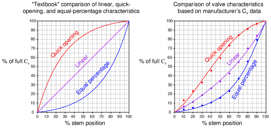
When we compare the performance of an equal-percentage control valve against the linear control valve from the previous scenario (where water flowed from a dam through a long, narrow pipe) using the “load line” plot to determine flow rates, we see that the equal-percentage valve yields a more linear installed response than the inherently linear valve. You can see how the blue curves on these graphs (representing each control valve’s Cv at 25%, 50%, 75%, and 100% stem positions) are identical only at the wide-open position and differ at all other positions:
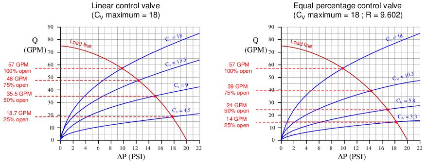
Note that the equal-percentage valve with a maximum Cv of 18 does not yield any greater water flow rate at full-open than the linear valve with the same maximum Cv. No amount or type of valve characterization can make up for the pressure lost in restrictive piping. What equal-percentage characterization does accomplish is to make the relationship between flow rate and stem position closer to linear than it would be otherwise.
Different valve characterizations are be achieved by different valve trim shapes. For instance, the plug profiles of a single-ported, stem-guided globe valve may be modified to achieve the common quick-opening, linear, and equal-percentage characteristics:
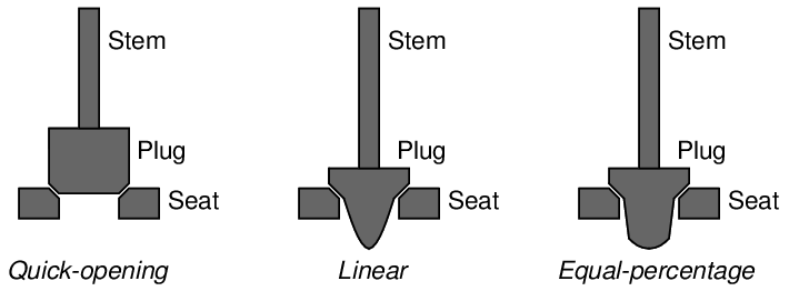
Photographs of linear (left) and equal-percentage (right) globe valve plugs having the same port size are shown side-by-side for comparison:
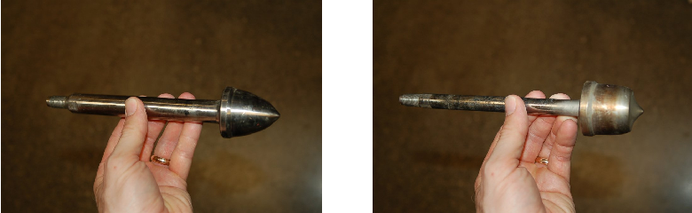
It should be clear46 how the equal-percentage plug on the right-hand side retains more of its width along its length than the linear plug on the left-hand side. This means the equal-percentage plug is more restrictive than the linear plug for a greater portion of its withdrawal out of the seat. As each plug is drawn out of the seat’s port by the actuator motion, the linear plug “opens up” more aggressively than the equal-percentage plug, even though both plugs are equally open when drawn fully out of the seat’s port.
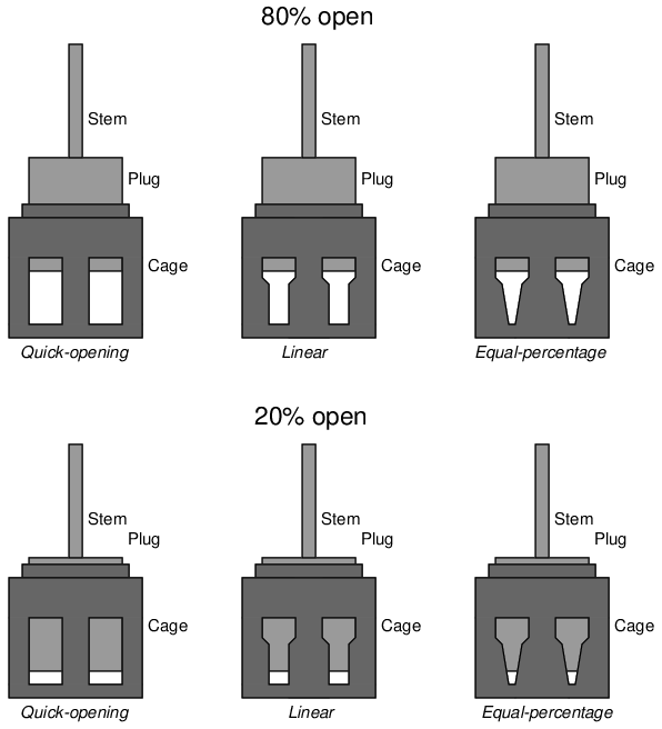
Cage-guided globe valve trim characteristic is a function of port shape. As the plug rises up, the amount of port area uncovered determines the shape of the characteristic graph:
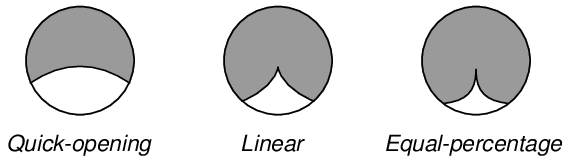
Ball valve trim characteristic is a function of notch shape. As the ball rotates, the amount of notch area opened to the fluid determines the shape of the characteristic graph. All valve trim in the following illustration is shown approximately half-open (50% stem rotation):
A different approach to valve characterization is to use a non-linear positioner function instead of a non-linear trim. That is, by “programming” a valve positioner to respond in a characterized fashion to command signals, it is possible to make an inherently linear valve behave as though it were quick-opening, equal-percentage, or anywhere in between. All the positioner does is modify the valve stem position as per the desired characteristic function instead of proportionally follow the signal as it normally would.
This approach has the distinct advantage of convenience (especially if the valve is already equipped with a positioner) over changing the actual valve trim. However, if valve stem friction ever becomes a problem, its effects will be disproportionate along the valve travel range, as the positioner must position the valve more precisely in some areas of travel than others when pressed into service as a characterizer.
It should be noted that not all process control loops benefit from control valves with equal-percentage inherent characteristics. There are some process applications, for example, where the pressure drop across a control valve holds relatively constant over a wide range of valve flow rates47 , in which case an inherently linear control valve will indeed yield a linear installed characteristic. In other words, if the pressure drop across the control valve never changes much, what we have is an “ideal” scenario (i.e. no “droop” or “distortion”) that doesn’t need special valve characterization to behave linearly.
Some other process applications actually work quite well48 with a quick-opening installed valve characteristic, in which case an inherently linear valve with varying pressure drop at different flow rates suffices. Ultimately, what matters is the valve stem position’s effect on the process variable and whether that relationship is consistent (linear) over a wide range of operating conditions.