
The two “process variables” we rely on most heavily in the field of electrical measurement and control are voltage and current. From these primary variables we may determine impedance, reactance, resistance, as well as the reciprocals of those quantities (admittance, susceptance, and conductance).
Other sensors more common to general process measurement such as temperature, pressure, level, and flow are also used in electric power systems, but their coverage in other chapters of this book is sufficient to avoid repetition in this chapter.
Two common types of electrical sensors used in the power industry are potential transformers (PTs) and current transformers (CTs). These are precision-ratio electromagnetic transformers used to step high voltages and high currents down to more reasonable levels for the benefit of panel-mounted instruments to receive, display, and/or process.
25.6.1 Potential transformers
Electrical power systems typically operate at dangerously high voltage. It would be both impractical and unsafe to connect panel-mounted instruments directly to the conductors of a power system if the voltage of that power system exceeds several hundred volts. For this reason, we must use a special type of step-down transformer referred to as a potential transformer to reduce and isolate the high line voltage of a power system to levels safe for panel-mounted instruments to input.
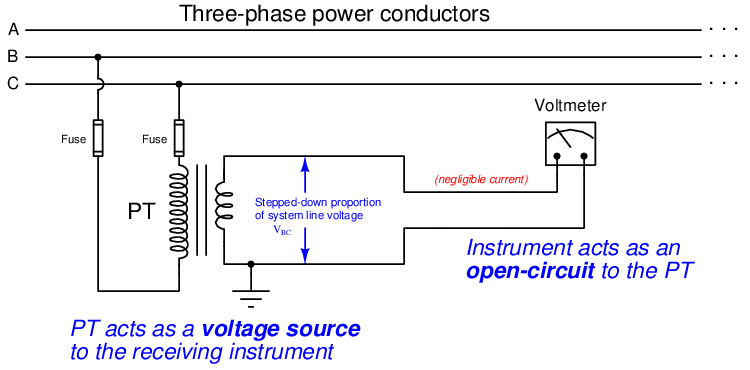
Shown here is a simple diagram illustrating how the high phase and line voltages of a three-phase AC power system may be sensed by low-voltage voltmeters through the use of step-down potential transformers:
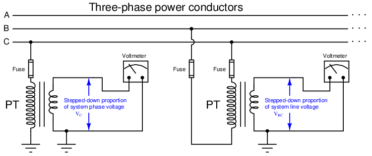
Potential transformers are commonly referred to as “PT” units in the electrical power industry. It should be noted that the term “voltage transformer” and its associated abbreviation VT is becoming popular as a replacement for “potential transformer” and PT.
When driving a voltmeter – which is essentially an open-circuit (very high resistance) – the PT behaves as a voltage source to the receiving instrument, sending a voltage signal to that instrument proportionately representing the power system’s voltage.
The following photograph shows a potential transformer sensing the phase-to-ground voltage on a three-phase power distribution system. The normal phase voltage in this system is 7.2 kV (12.5 kV three-phase line voltage), and the PT’s normal secondary voltage is 120 volts, necessitating a ratio of 60:1 (as shown on the transformer’s side):
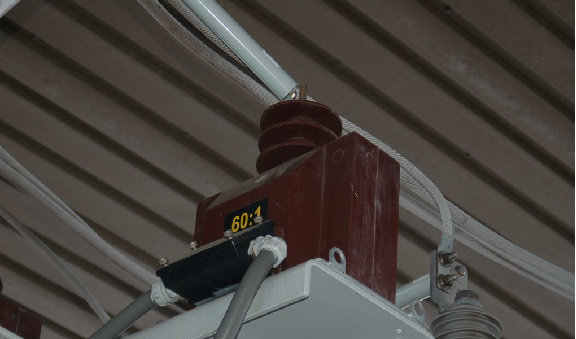
Any voltage output by this PT will be 1 _ 60 of the actual phase voltage, allowing panel-mounted instruments to read a precisely scaled proportion of the 7.2 kV (typical) phase voltage safely and effectively. A panel-mounted voltmeter, for example, would have a scale registering 7200 volts when its actual input terminal voltage was only 120 volts. This is analogous to a 4-20 mA indicating meter bearing a scale labeled in units of “PSI” or “Degrees Celsius” because the 4-20 mA analog signal merely represents some other physical variable sensed by a process transmitter. Here, the physical variable being sensed by the potential transformer is still voltage, just at a 60:1 ratio greater than what the panel-mounted instrument receives. Like the 4-20 mA DC analog signal standard so common in the process industries, 115 or 120 volts is the standard potential transformer output voltage used in the electrical industry to represent normal power system voltage.
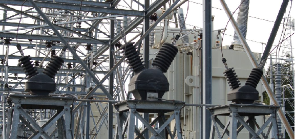
This next photograph shows a set of three PTs used to measure voltage on a 13.8 kV substation bus. Note how each of these PTs is equipped with two high-voltage insulated terminals to facilitate phase-to-phase (line voltage) measurements as well as phase-to-ground:
Another photograph of potential transformers appears here, showing three large PTs used to precisely step the phase-to-ground voltages for each phase of a 230 kV system (230 kV line voltage, 133 kV phase voltage) all the way down to 120 volts for the panel-mounted instruments to monitor:
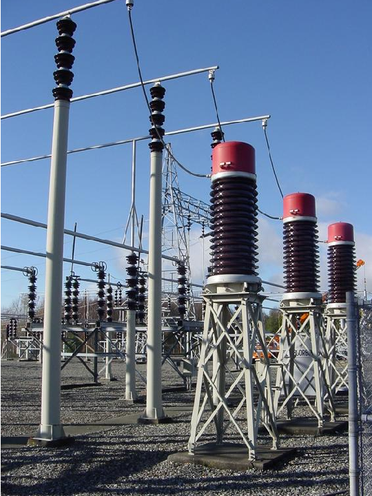
A loose-hanging wire joins one side of each PT’s primary winding to the respective phase conductor of the 230 kV bus. The other terminal of each PT’s primary winding connects to a common neutral point, forming a Wye-connected PT transformer array. The secondary terminals of these PTs connect to two-wire shielded cables conveying the 120 volt signals back to the control room where they terminate at various instruments. These shielded cables run through underground conduit for protection from weather.
Just as with the previous PT, the standard output voltage of these large PTs is 120 volts, equating to a transformer turns ratio of about 1100:1. This standardized output voltage of 120 volts allows PTs of any manufacture to be used with receiving instruments of any manufacture, just as the 4-20 mA standard for analog industrial instruments allows “interoperability” between different manufacturers’ brands and models.
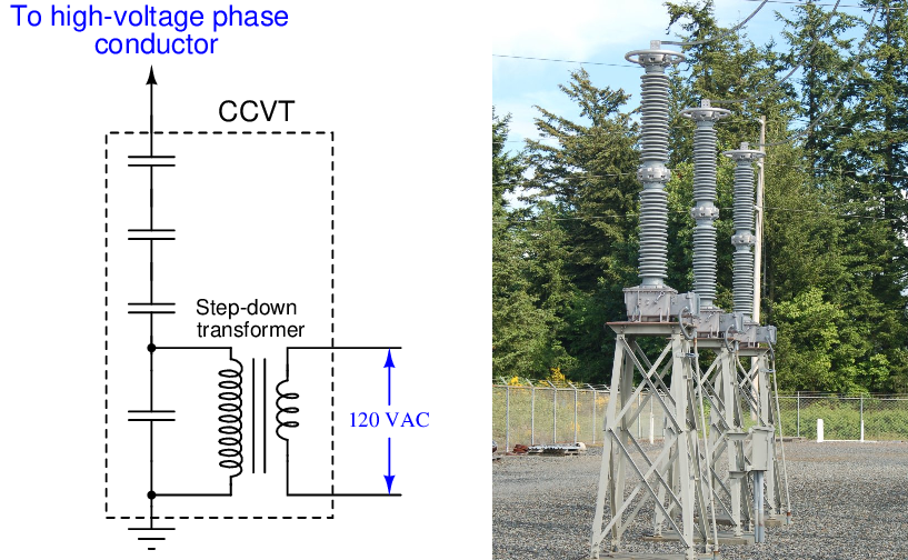
A special form of instrument transformer used on very high-voltage systems is the capacitively-coupled voltage transformer, or CCVT. These sensing devices employ a series-connected set of capacitors dividing the power line voltage down to a lesser quantity before it gets stepped down further by an electromagnetic transformer. A simplified diagram of a CCVT appears here, along with a photograph of three CCVTs located in a substation:
25.6.2 Current transformers
For the same reasons necessitating the use of potential (voltage) instrument transformers, we also see the use of current transformers to reduce high current values and isolate high voltage values between the electrical power system conductors and panel-mounted instruments.
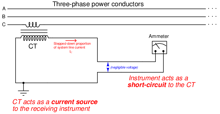
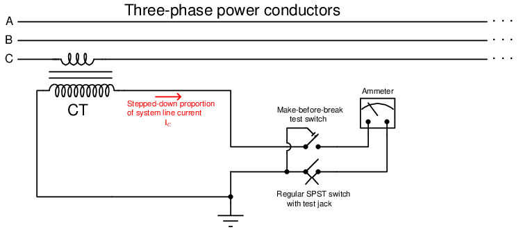
Shown here is a simple diagram illustrating how the line current of a three-phase AC power system may be sensed by a low-current ammeter through the use of a current transformer:
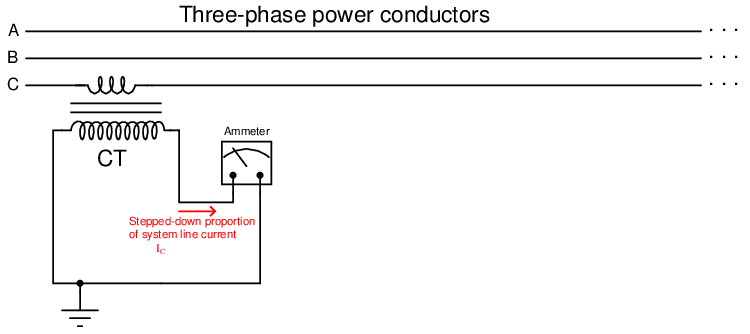
When driving an ammeter – which is essentially a short-circuit (very low resistance) – the CT behaves as a current source to the receiving instrument, sending a current signal to that instrument proportionately representing the power system’s line current.
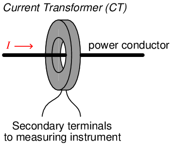
In typical practice a CT consists of an iron toroid25 functioning as the transformer core. This type of CT does not have a primary “winding” in the conventional sense of the word, but rather uses the line conductor itself as the primary winding. The line conductor passing once through the center of the toroid functions as a primary transformer winding with exactly 1 “turn”. The secondary winding consists of multiple turns of wire wrapped around the toroidal magnetic core:
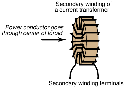
A view of a current transformer’s construction shows the wrapping of the secondary turns around the toroidal magnetic core in such a way that the secondary conductor remains parallel to the primary (power) conductor for good magnetic coupling:
With the power conductor serving as a single-turn26 winding, the multiple turns of secondary wire around the toroidal core of a CT makes it function as a step-up transformer with regard to voltage, and as a step-down transformer with regard to current. The turns ratio of a CT is typically specified as a ratio of full line conductor current to 5 amps, which is a standard output current for power CTs. Therefore, a 100:5 ratio CT outputs 5 amps when the power conductor carries 100 amps.
The turns ratio of a current transformer suggests a danger worthy of note: if the secondary winding of an energized CT is ever open-circuited, it may develop an extremely high voltage as it attempts to force current through the air gap of that open circuit. An energized CT secondary winding acts like a current source, and like all current sources it will develop as great a potential (voltage) as it can when presented with an open circuit. Given the high voltage capability of the power system being monitored by the CT, and the CT turns ratio with more turns in the secondary than in the primary, the ability for a CT to function as a voltage step-up transformer poses a significant hazard.
Like any other current source, there is no harm in short-circuiting the output of a CT. Only an open circuit poses risk of damage. For this reason, CT circuits are often equipped with shorting bars and/or shorting switches to allow technicians to place a short-circuit across the CT secondary winding before disconnecting any other wires in the circuit. Later subsections will elaborate on this topic in greater detail.
Current transformers are manufactured in a wide range of sizes, to accommodate different applications. Here is a photograph of a current transformer showing the “nameplate” label with all relevant specifications. This nameplate specifies the current ratio as “100/5” which means this CT will output 5 amps of current when there is 100 amps flowing through a power conductor passed through the center of the toroid:
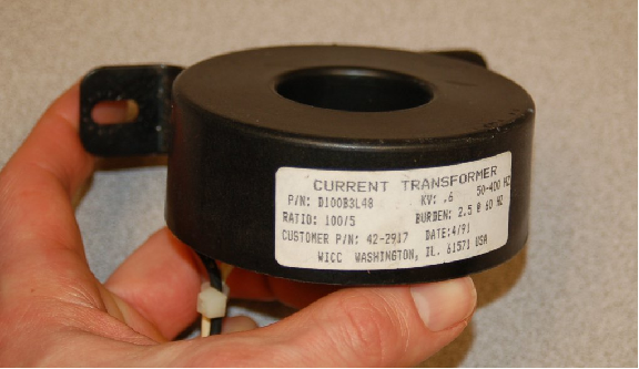
The black and white wire pair exiting this CT carries the 0 to 5 amp AC current signal to any monitoring instrument scaled to that range. That instrument will see 1 _ 20 (i.e. 5 _ 100) of the current flowing through the power conductor.
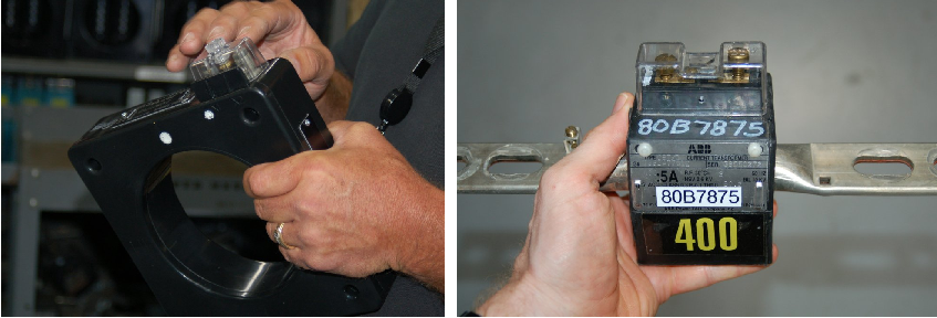
The following photographs contrast two different styles of current transformer, one with a “window” through which any conductor may be passed, and another with a dedicated busbar fixed through the center to which conductors attach at either end. Both styles are commonly found in the electrical power industry, and they operate identically:
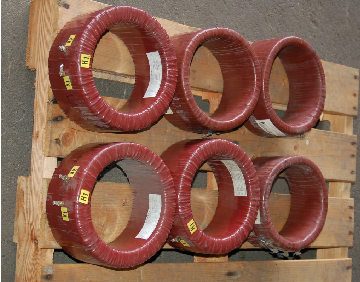
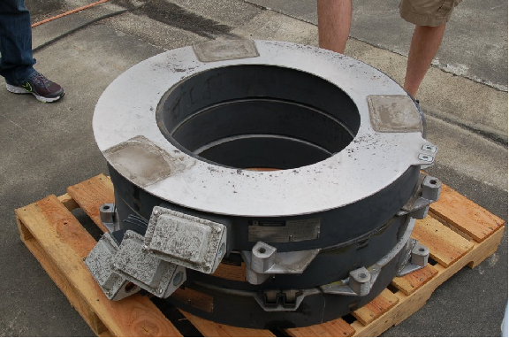
Here is a photograph of some much larger CTs intended for installation inside the “bushings27 ” of a large circuit breaker, stored on a wooden pallet:
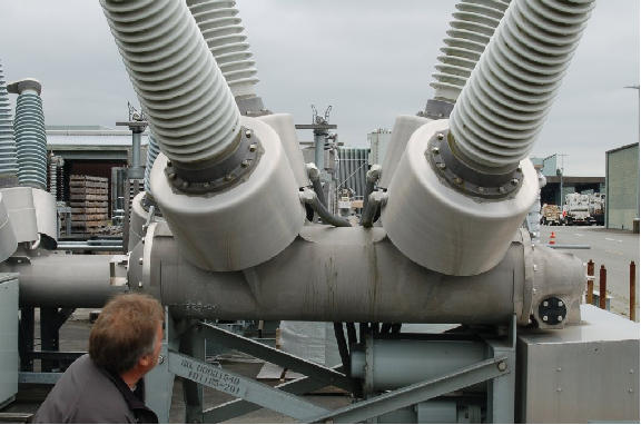
The installed CTs appear as cylindrical bulges at the base of each insulator on the high-voltage circuit breaker. This particular photograph shows flexible conduit running to each bushing CT, carrying the low-current CT secondary signals to a terminal strip inside a panel on the right-hand end of the breaker:
Signals from the bushing CTs on a circuit breaker may be connected to protective relay devices to trip the breaker in the event of any abnormal condition. If unused, a CT’s secondary terminals are simply short-circuited at the panel.
Shown here is a set of three very large CTs, intended for installation at the bushings of a high-voltage power transformer. Each one has a current step-down ratio of 600-to-5:
In this next photograph we see a tiny CT designed for low current measurements, clipped over a wire carrying only a few amps of current. This particular current transformer is constructed in such a way that it may be clipped around an existing wire for temporary test purposes, rather than being a solid toroid where the conductor must be threaded through it for a more permanent installation:
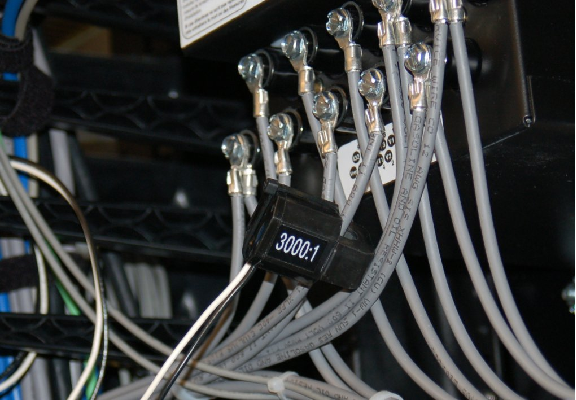
This CT’s ratio of 3000:1 would step down a 5 amp AC signal to 1.667 milliamps AC.
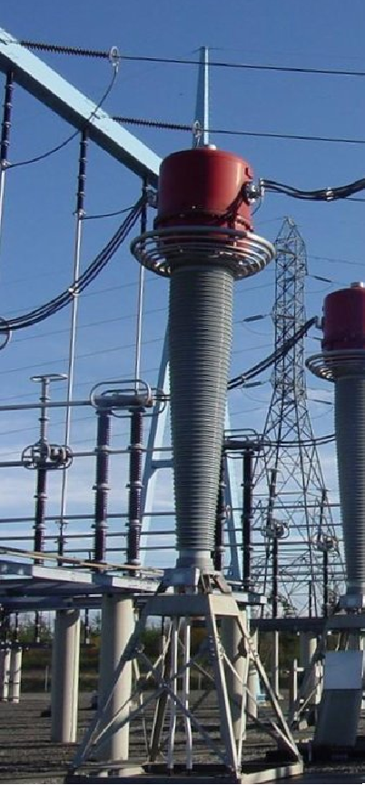
This last photograph shows a current transformer used to measure line current in a 500 kV substation switchyard. The actual CT coil is located inside the red-colored housing at the top of the insulator, where the power conductor passes through. The tall insulator stack provides necessary separation between the conductor and the earth below to prevent high voltage from “jumping” to ground through the air:
25.6.3 Transformer polarity
An important characteristic to identify for transformers in power systems – both power transformers and instrument transformers – is polarity. At first it may seem inappropriate to speak of “polarity” when we know we are dealing with alternating voltages and currents, but what is really meant by this word is phasing. When multiple power transformers are interconnected in order to share load, or to form a three-phase transformer array from three single-phase transformer units, it is critical that the phase relationships between the transformer windings be known and clearly marked. Also, we need to know the phase relationship between the primary and secondary windings (coils) of an instrument transformer in order to properly connect it to a receiving instrument such as a protective relay. For some instruments such as simple indicating meters, polarity (phasing) is unimportant. For other instruments comparing the phase relationships of two or more received signals from instrument transformers, proper polarity (phasing) is critical.
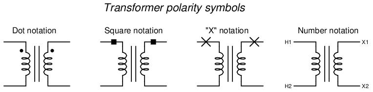
Polarity markings for any transformer may be symbolized several different ways:
The marks should be interpreted in terms of voltage polarity, not current. To illustrate using a “test circuit28 ” feeding a momentary pulse of DC to a transformer from a small battery:
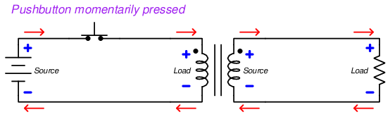
Note how the secondary winding of the transformer develops the same polarity of voltage drop as is impressed across the primary winding by the DC pulse: for both the primary and secondary windings, the sides with the dots share the same positive potential.
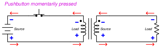
If the battery were reversed and the test performed again, the side of each transformer winding with the dot would be negative:
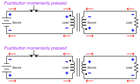
If we reverse the secondary winding’s connection to the resistor and re-draw all voltages and currents, we see that the polarity dot always represents common voltage potential, regardless of source polarity:
It should be noted that this battery-and-switch method of testing should employ a fairly low-voltage battery in order to avoid leaving residual magnetism in the transformer’s core29 . A single 9-volt dry-cell battery works well given a sensitive meter.
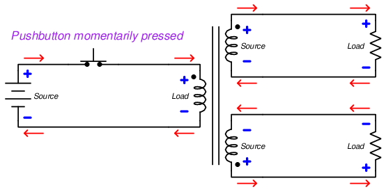
Transformers with multiple secondary windings act the same, with each secondary winding’s polarity mark having the same polarity as every other winding:
To emphasize this important point again: transformer polarity dots always refer to voltage, never current. The polarity of voltage across a transformer winding will always match the polarity of every other winding on that same transformer in relation to the dots. The direction of current through a transformer winding, however, depends on whether the winding in question is functioning as a source or a load. This is why currents are seen to be in opposite directions (into the dot, out of the dot) from primary to secondary in all the previous examples shown while the voltage polarities all match the dots. A transformer’s primary winding functions as a load (conventional-flow current drawn flowing into the positive terminal) while its secondary winding functions as a source (conventional-flow current flowing out of the positive terminal).
Transformer polarity is very important in the electric power industry, and so terms have been coined for different polarity orientations of transformer windings. If polarity dots for primary and secondary windings lie on the same physical side of the transformer it means the primary and secondary windings are wrapped the same direction around the core, and this is called a subtractive transformer. If polarity dots lie on opposite sides of the transformer it means the primary and secondary windings are wrapped in opposite directions, and this is called an additive transformer. The terms “additive” and “subtractive” have more meaning when we view the effects of each configuration in a grounded AC power system. The following examples show how voltages may either add or subtract depending on the phase relationships of primary and secondary transformer windings:
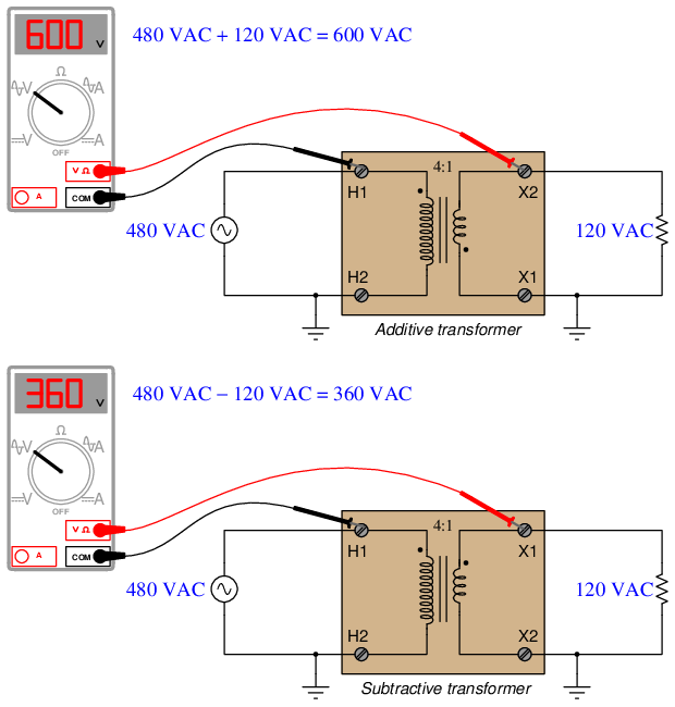
Transformers operating at high voltages are typically designed with subtractive winding30 orientations, simply to minimize the dielectric stress placing on winding insulation from inter-winding voltages. Instrument transformers (PTs and CTs) by convention are always subtractive.
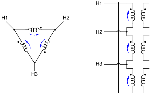
When three single-phase transformers are interconnected to form a three-phase transformer bank, the winding polarities must be properly oriented. Windings in a delta network must be connected such that the polarity marks of no two windings are common to each other. Curved arrows are drawn next to each winding to emphasize the phase relationships:
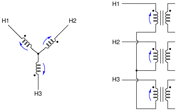
Windings in a wye network must be connected such that the polarity marks all face the same direction with respect to the center of the wye (typically, the polarity marks are all facing away from the center):
Failure to heed these phase relationships in a power transformer bank may result in catastrophic failure as soon as the transformers are energized!
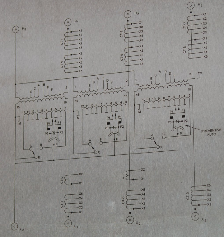
The following photograph shows the diagram for a large utility power transformer31 equipped with a number of current transformers permanently installed in the bushings (the points at which power conductors penetrate the steel casing of the power transformer unit). Note the solid black squares marking one side of each CT secondary winding as well as one side of each primary and secondary winding in this three-phase power transformer. Comparing placement of these black squares we can tell all CTs as well as the power transformer itself are wound as subtractive devices:
An example of the importance of polarity marks to the connection of instrument transformers may be seen here, where a pair of current transformers with equal turns ratios are connected in parallel to drive a common instrument which is supposed to measure the difference in current entering and exiting a load:
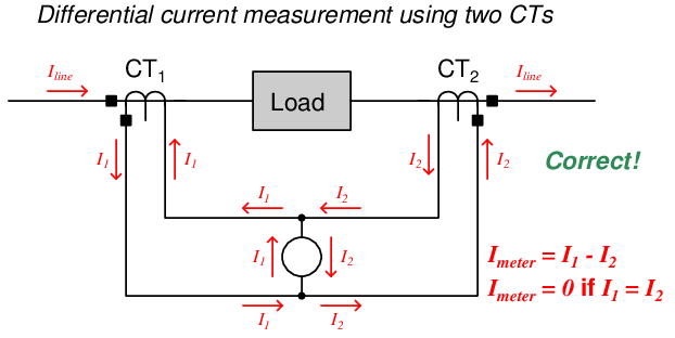
Properly connected as shown above, the meter in the center of the circuit registers only the difference in current output by the two current transformers. If current into the load is precisely equal to current out of the load (which it should be), and the two CTs are precisely matched in their turns ratio, the meter will receive zero net current. If, however, a ground fault develops within the load causing more current to enter than to exit it, the imbalance in CT currents will be registered by the meter and thus indicate a fault condition in the load.
Let us suppose, though, that a technician mistakenly connected one of these CT units backwards. If we examine the resulting circuit, we see that the meter now senses the sum of the line currents rather than the difference as it should:
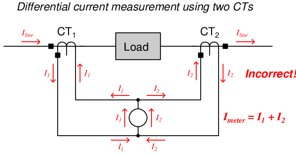
This will cause the meter to falsely indicate a current imbalance in the load when none exists.
25.6.4 Instrument transformer safety
Potential transformers (PTs or VTs) tend to behave as voltage sources to the voltage-sensing instruments they drive: the signal output by a PT is supposed to be a proportional representation of the power system’s voltage. Conversely, current transformers (CTs) tend to behave as current sources to the current-sensing instruments they drive: the signal output by a CT is supposed to be a proportional representation of the power system’s current. The following schematic diagrams show how PTs and CTs should behave when sourcing their respective instruments:
In keeping with this principle of PTs as voltage sources and CTs as current sources, a PT’s secondary winding should never be short-circuited and a CT’s secondary winding should never be open-circuited! Short-circuiting a PT’s secondary winding may result in a dangerous amount of current developing in the circuit because the PT will attempt to maintain a substantial voltage across a very low resistance. Open-circuiting a CT’s secondary winding may result in a dangerous amount of voltage32 developing between the secondary terminals because the CT will attempt to drive a substantial current through a very high resistance.
This is why you will never see fuses in the secondary circuit of a current transformer. Such a fuse, when blown open, would pose a greater hazard to life and property than a closed circuit with any amount of current the CT could muster.
While the recommendation to never short-circuit the output of a PT makes perfect sense to any student of electricity or electronics who has been drilled never to short-circuit a battery or a laboratory power supply, the recommendation to never open-circuit a powered CT often requires some explanation. Since CTs transform current, their output current value is naturally limited to a fixed ratio of the power conductor’s line current. That is to say, short-circuiting the secondary winding of a CT will not result in more current output by that CT than what it would output to any normal current-sensing instrument! In fact, a CT encounters minimum “burden” when powering a short-circuit because it doesn’t have to output any substantial voltage to maintain that amount of secondary current. It is only when a CT is forced to output current through a substantial impedance that it must “work hard” (i.e. output more power) by generating a substantial secondary voltage along with a secondary current.
The latent danger of a CT is underscored by an examination of its primary-to-secondary turns ratio. A single conductor passed through the aperture of a current transformer acts as a winding with one turn, while the multiple turns of wire wrapped around the toroidal core of a current transformer provides the ratio necessary to step down current from the power line to the receiving instrument. However, as every student of transformers knows, while a secondary winding possessing more turns of wire than the primary steps current down, that same transformer conversely will step voltage up. This means an open-circuited CT behaves as a voltage step-up transformer. Given the fact that the power line being measured usually has a dangerously high voltage to begin with, the prospect of an instrument transformer stepping that voltage up even higher is sobering indeed. In fact, the only way to ensure a CT will not output high voltage when powered by line current is to keep its secondary winding loaded with a low impedance.
It is also imperative that all instrument transformer secondary windings be solidly grounded to prevent dangerously high voltages from developing at the instrument terminals via capacitive coupling with the power conductors. Grounding should be done at only one point in each instrument transformer circuit to prevent ground loops from forming and potentially causing measurement errors. The preferable location of this grounding is at the first point of use, i.e. the instrument or panel-mounted terminal block where the instrument transformer’s secondary wires land. If any test switches exist between the instrument transformer and the receiving instrument, the ground connection must be made in such a way that opening the test switch does not leave the transformer’s secondary winding floating (ungrounded).
25.6.5 Instrument transformer test switches
Connections made between instrument transformers and receiving instruments such as panel-mounted meters and relays must be occasionally broken in order to perform tests and other maintenance functions. An accessory often seen in power instrument panels is a test switch bank, consisting of a series of knife switches. A photograph of a test switch bank manufactured by ABB is seen here:
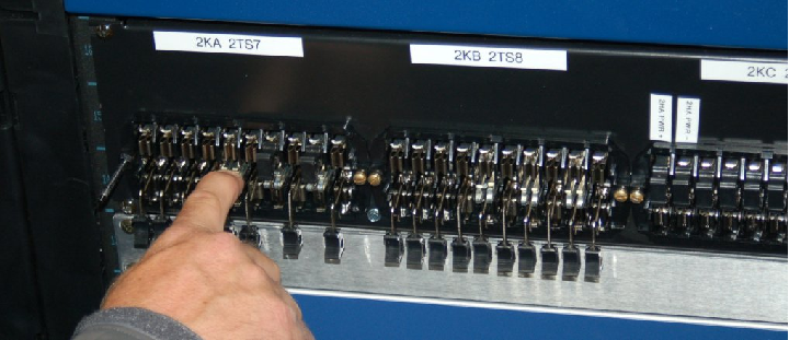
Some of these knife switches serve to disconnect potential transformers (PTs) from receiving instruments mounted on this relay panel, while other knife switches in the same bank serve to disconnect current transformers (CTs) from receiving instruments mounted on the same panel.
For added security, covers may be installed on the switch bank to prevent accidental operation or electrical contact. Some test switch covers are even lock-able by padlock, for an added measure of access prevention.
Test switches used to disconnect potential transformers (PTs) from voltage-sensing instruments are nothing more than simple single-pole, single-throw (SPST) knife switches, as shown in this diagram:
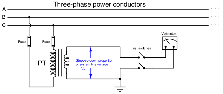
There is no danger in open-circuiting a potential transformer circuit, and so nothing special is needed to disconnect a PT from a receiving instrument.
A series of photographs showing the operation of one of these knife switches appears here, from closed (in-service) on the left to open (disconnected) on the right:
Test switches used to disconnect current transformers (CTs) from current-sensing instruments, however, must be specially designed to avoid opening the CT circuit when disconnecting, due to the high-voltage danger posed by open-circuited CT secondary windings. Thus, CT test switches are designed to place a short-circuit across the CT’s output before opening the connection to the current-measuring device. This is done through the use of a special make-before-break knife switch:
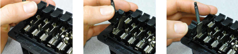
A series of photographs showing the operation of a make-before-break knife switch appears here, from closed (in-service) on the left to shorted (disconnected) on the right:
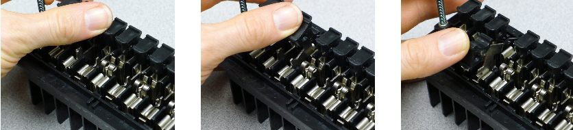
The shorting action takes place at a spring-steel leaf contacting the moving knife blade at a cam cut near the hinge. Note how the leaf is contacting the cam of the knife in the right-hand and middle photographs, but not in the left-hand photograph. This metal leaf joins with the base of the knife switch adjacent to the right (the other pole of the CT circuit), forming the short-circuit between CT terminals necessary to prevent arcing when the knife switch opens the circuit to the receiving instrument.
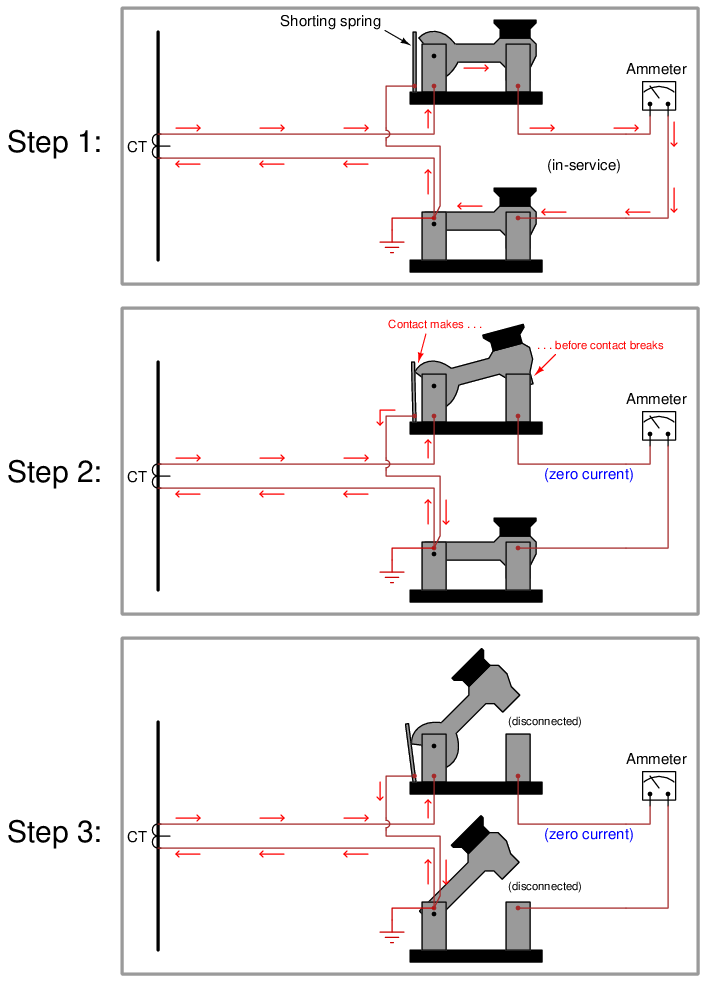
A step-by-step sequence of illustrations shows how this shorting spring works to prevent the CT circuit from opening when the first switch is opened:
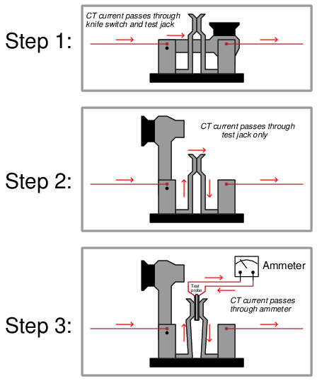
It is typical that the non-shorting switch in a CT test switch pair be equipped with a “test jack” allowing the insertion of an additional ammeter in the circuit for measurement of the CT’s signal. This test jack consists of a pair of spring-steel leafs contacting each other in the middle of the knife switch’s span. When that knife switch is in the open position, the metal leafs continue to provide continuity past the open knife switch. However, when a special ammeter adapter plug is forced between the leafs, spreading them apart, the circuit breaks and the current must flow through the two prongs of the test plug (and to the test ammeter connected to that plug).
A step-by-step sequence of illustrations shows how a test jack maintains continuity across an opened knife switch, and then allows the insertion of a test probe and ammeter, without ever breaking the CT circuit:
When using a CT test probe like this, one must be sure to thoroughly test the electrical continuity of the ammeter and test leads before inserting the probe into the test jacks. If there happens to be an “open” fault anywhere in the ammeter/lead circuit, a dangerous arc will develop at the point of that “open” the moment the test probe forces the metal leafs of the test jack apart! Always remember that a live CT is dangerous when open-circuited, and so your personal safety depends on always maintaining electrical continuity in the CT circuit.
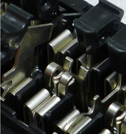
This close-up photograph shows a closed CT test switch equipped with a test jack, the jack’s spring leafs visible as a pair of “hoop” shaped structures flanking the blade of the middle knife switch:
In addition to (or sometimes in lieu of) test switches, current transformer secondary wiring often passes through special “shorting” terminal blocks. These special terminal blocks have a metal “shorting bar” running down their center, through which screws may be inserted to engage with wired terminals below. Any terminals made common to this metal bar will necessarily be equipotential to each other. One screw is always inserted into the bar tapping into the earth ground terminal on the terminal block, thus making the entire bar grounded. Additional screws inserted into this bar force CT secondary wires to ground potential. A photo of such a shorting terminal block is shown here, with five conductors from a multi-ratio (multi-tap) current transformer labeled 7X1 through 7X5 connecting to the terminal block from below:
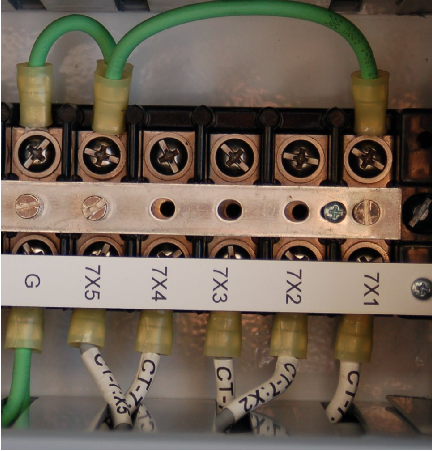
This shorting terminal block has three screws inserted into the shorting bar: one bonding the bar to the ground (“G”) terminal on the far-left side, another one connecting to the “7X5” CT wire, and the last one connecting to the “7X1” CT wire. While the first screw establishes earth ground potential along the shorting bar, the next two screws form a short circuit between the outer two conductors of the multi-ratio current transformer. Note the green “jumper” wires attached to the top side of this terminal block shorting 7X1 to 7X5 to ground, as an additional measure of safety for this particular CT which is currently unused and not connected to any measuring instrument.
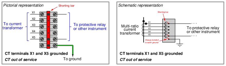
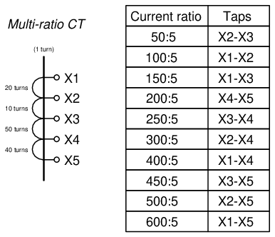
The following illustrations show combinations of screw terminal positions used to selectively ground different conductors on a multi-ratio current transformer. The first of these illustrations show the condition represented in the previous photograph, with the entire CT shorted and grounded:
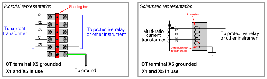
This next illustration shows how the CT would be used in its full capacity, with X1 and X5 connecting to the panel instrument and (only) X5 grounded for safety:
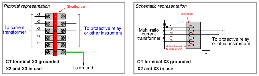
This final illustration shows how the CT would be used in reduced capacity, with X2 and X3 connecting to the panel instrument and (only) X3 grounded for safety:
25.6.6 Instrument transformer burden and accuracy
In order for an instrument transformer to function as an accurate sensing device, it must not be unduly tasked with delivering power to a load. In order to minimize the power demand placed on instrument transformers, an ideal voltage-measuring instrument should draw zero current from its PT, while an ideal current-measuring instrument should drop zero voltage across its CT.
The goal of delivering zero power to any instrument is difficult to achieve in practice. Every voltmeter does indeed draw some current, however slight. Every ammeter does drop some voltage, however slight. The amount of apparent power drawn from any instrument transformer is appropriately called burden, and like all expressions of apparent power is measured in units of volt-amps. The greater this burden, the more the instrument transformer’s signal will “sag” (decrease from loading). Therefore, minimizing burden is a matter of maximizing accuracy for power system measurement.
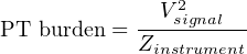
The burden value for any instrument transformer is a function of apparent power, impedance, and either voltage or current according to the familiar apparent power formulae S = V 2 Z and S = I2Z:

Burden for any device or circuit connected to an instrument transformer may be expressed as an impedance value (Z) in ohms, or as an apparent power value (S) in volt-amps. Similarly, instrument transformers themselves are usually rated for the amount of burden they may source and still perform within a certain accuracy tolerance (e.g. ± 1% at a burden of 2 VA).
Potential transformer burden and accuracy ratings
Potential transformers have maximum burden values specified in terms of apparent power (S,measured in volt-amps), standard burden values being classified by letter code:
| Letter code | Maximum allowable burden at stated accuracy |
| W | 12.5 volt-amps |
| X | 25 volt-amps |
| M | 35 volt-amps |
| Y | 75 volt-amps |
| Z | 200 volt-amps |
| ZZ | 400 volt-amps |
Standard accuracy classes for potential transformers include 0.3, 0.6, and 1.2, corresponding to uncertainties of ± 0.3%, ± 0.6%, and ± 1.2% of the rated turns ratio, respectively. These accuracy class and burden ratings are typically combined into one label. A potential transformer rated “0.6M” therefore has an accuracy of ± 0.6% (this percentage being understood as its turns ratio accuracy) while powering a burden of 35 volt-amps at its nominal (e.g. 120 volts) output.
Current transformer burden and accuracy ratings
Current transformer accuracies and burdens are more complicated than potential transformer ratings. The principal reason for this is the wider range of CT application. If a current transformer is to be used for metering purposes (i.e. driving wattmeters, ammeters, and other instruments used for regulatory control and/or revenue billing where high accuracy is required), it is assumed the transformer will operate within its standard rated current values. For example, a 600:5 ratio current transformer used for metering should rarely if ever see a primary current value exceeding 600 amps, or a secondary current exceeding 5 amps. If current values through the CT ever do exceed these maximum standard values, the effect on regulation or billing will be negligible because these should be transient events. However, protective relays are designed to interpret and act upon transient events in power systems. If a current transformer is to be used for relaying rather than metering, it must reliably perform under overload conditions typically created by power system faults. In other words, relay applications of CTs demand a much larger dynamic range of measurement than meter applications. Absolute accuracy is not as important for relays, but we must ensure the CT will give a reasonably accurate representation of line current during fault conditions in order for the protective relay(s) to function properly. PTs, even those used for protective relaying purposes, never see voltage transients as wide-ranging as the current transients seen by CTs.
Meter class CT ratings typically take the form of a percentage value followed by the letter “B” followed by the maximum burden expressed in ohms of impedance. Therefore, a CT with a metering classification of 0.3B1.8 exhibits an accuracy of ± 0.3% of turns ratio when powering a 1.8 ohm meter impedance at 100% output current (typically 5 amps).
Relay class CT ratings typically take the form of a maximum voltage value dropped across the burden at 20 times rated current (i.e. 100 amps secondary current for a CT with a 5 amp nominal output rating) while maintaining an accuracy within ±10% of the rated turns ratio. Not coincidentally, this is how CT ratios are usually selected for power system protection: such that the maximum expected symmetrical fault current through the power conductor does not exceed 20 times the primary current rating of the CT33 . Therefore, a CT with a relay classification of C200 is able to output up to 200 volts while powering its maximum burden at 20× rated current. Assuming a rated output current of 5 amps, 20 times this value would be 100 amps delivered to the relay. If the relay’s voltage drop at this current is allowed to be as high as 200 volts, it means the CT secondary circuit may have an impedance value of up to 2 ohms (200 V ÷ 100 A = 2 Ω). Therefore, a relaying CT rating of C200 is just another way of saying it can power as much as 2 ohms of burden.
The letter “C” in the “C200” rating example stands for calculated, which means the rating is based on theory. Some current transformers use the letter “T” instead, which stands for tested. These CTs have been actually tested at the specified voltage and current values to ensure their performance under real-world conditions.
Current transformer saturation
It is worthwhile to explore the concept of maximum CT burden in some detail. In an ideal world, a CT acts as a current source to the meter or relay it is powering, and as such it is quite content to drive current into a short circuit (0 ohms impedance). Problems arise if we demand the CT to supply more power than it is designed to, which means forcing the CT to drive current through an excessive amount of impedance. In the days of electromechanical meters and protective relays where the devices were entirely powered by instrument transformer signals, the amount of burden imposed by certain meters and relays could be quite substantial34 . Modern electronic meters and relays pose much less burden to instrument transformers, approaching the ideal conditions of zero impedance for current-sensing inputs.
The voltage developed by any inductance, including transformer windings, is described by Faraday’s Law of Electromagnetic Induction:

Where,
V = Induced voltage (volts)
N = Number of turns of wire
dϕ__ dt = Rate of change of magnetic flux (Webers per second)
To generate a larger voltage, therefore, a current transformer must develop a faster-changing magnetic flux in its core. If the voltage in question is sinusoidal at a constant frequency, the magnetic flux also traces a sinusoidal function over time, the voltage peaks coinciding with the steepest points on the flux waveform, and the voltage “zero” points coinciding with the peaks on the flux waveform where the rate-of-change of magnetic flux over time is zero:
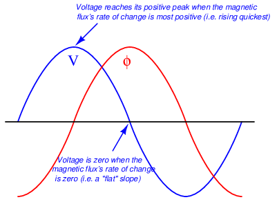
Imposing a larger burden on a CT (i.e. more impedance the current must drive through) means the CT must develop a larger sinusoidal voltage for any given amount of measured line current. This equates to a flux waveform with a faster-changing rate of rise and fall, which in turn means a higher-peak flux waveform (assuming a sinusoidal shape). The problem with this at some point is that the required magnetic flux reaches such high peak values that the ferrous35 core of the CT begins to saturate with magnetism, at which point the CT ceases to behave in a linear fashion and will no longer faithfully reproduce the shape and magnitude of the power line current waveform. In simple terms, if we place too much burden on a CT it will begin to output a distorted signal no longer faithfully representing line current.
The fact that a CT’s maximum AC voltage output depends on the magnetic saturation limit of its ferrous core becomes particularly relevant to multi-ratio CTs where the secondary winding is provided with more than two “taps”. Multi-ratio current transformers are commonly found as the permanently mounted CTs in the bushings of power transformers, giving the end-user freedom in configuring their metering and protection circuits. Consider this distribution transformer bushing 600:5 CT with a C800 accuracy class rating:
This CT’s “C800” classification is based on its ability to source a maximum of 800 volts to a burden when all of its secondary turns are in use. That is to say, its rating is “C800” only when connected to taps X1 and X5 for the full 600:5 ratio. If someone happens to connect to taps X1-X3 instead, using only 30 turns of wire in the CT’s secondary instead of all 120 turns, this CT will be limited to sourcing 200 volts to a burden before saturating: the same magnitude of magnetic flux that could generate 800 volts across 120 turns of wire can only induce one-quarter as much voltage across one-quarter the number of turns, in accordance with Faraday’s Law of Electromagnetic Induction (V = N dϕ dt ). Thus, the CT must be treated as a “C200” unit when wired for a 150:5 ratio.
The presence of any direct current in AC power line conductors poses a problem for current transformers which may only be understood in terms of magnetic flux in the CT core. Any direct current (DC) in a power line passing through a CT biases the CT’s magnetic field by some amount, making CT saturate more easily in one half-cycle of the AC than the other. Direct currents never sustain indefinitely in AC power systems, but are often present as transient pulses during certain fault conditions. Even so, transient DC currents will leave CT cores with some residual magnetic bias predisposing them to saturation in future fault conditions. The ability of a CT core to retain some magnetic flux over time is called remanence.
Remanence in a transformer core is an undesirable property. It may be mitigated by designing the core with a air gap (rather than making the core as an unbroken path of ferrous metal), but this compromises other desirable properties such as saturation limits (i.e. maximum output voltage). Some industry experts advise CTs be demagnetized by maintenance personnel as part of the repair work following a high-current fault, in order to ensure optimum performance when the system is returned to service. Demagnetization consists of passing a large AC current through the CT and then slowly reducing the magnitude of that AC current to zero amps. The gradual reduction of alternating magnetic field strength from full to zero tends to randomize the magnetic domains in the ferrous core, returning it to an unmagnetized state.
Whatever the cause, CT saturation can be a significant problem for protective relay circuits because these relays must reliably operate under all manner of transient overcurrent events. The more current through the primary of a CT, the more current it should output to the protective relay. For any given amount of relay burden (relay input impedance), a greater current signal translates into a greater voltage drop and therefore a greater demand for the CT to output a driving voltage. Thus, CT saturation is more likely to occur during overcurrent events when we most need the CT to function properly. Anyone tasked with selecting an appropriate current transformer for a protective relaying application must therefore carefully consider the maximum expected value of overcurrent for system faults, ensuring the CT(s) will do their job while driving the burdens imposed by the relays.
Current transformer testing
Current transformers may be bench-tested for turns ratio and saturation36 by applying a variable AC voltage to the secondary winding while monitoring secondary current and primary voltage. For common “window” style CTs, the primary winding is a single wire threaded through its center hole. An ideal current transformer would present a constant impedance to the AC voltage source and a constant voltage ratio from input to output. A real current transformer will exhibit less and less impedance as voltage is increased past its saturation threshold:
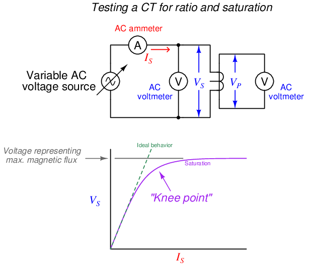
An ideal CT (with no saturation) would trace a straight line. The bent shape reveals the effects of magnetic saturation, where there is so much magnetism in the CT’s core that additional current only yields miniscule increases in magnetic flux (revealed by voltage drop).
Of course, a CT is never powered by its secondary winding when installed and operating. The purpose of powering a CT “backwards” as shown is to avoid having to drive very high currents through the primary of the CT. If high-current test equipment is available, however, such a primary injection test is actually the most realistic way to test a CT.
The following table shows actual voltage and current values taken during a secondary excitation test on a C400 class relay CT with a 2000:5 ratio. The source voltage was increased from zero to approximately 600 volts AC at 60 Hz for the test while secondary voltage drop and primary voltage were measured. Around 575 volts a “buzzing” sound could be heard coming from the CT – an audible effect of magnetic saturation. Calculated values of secondary winding impedance and turns ratio are also shown in this table:
| IS | V S | V P | ZS = V S ÷ IS | Ratio = V S ÷ V P |
| 0.0308 A | 75.14 V | 0.1788 V | 2.44 kΩ | 420.2 |
| 0.0322 A | 100.03 V | 0.2406 V | 3.11 kΩ | 415.8 |
| 0.0375 A | 150.11 V | 0.3661 V | 4.00 kΩ | 410.0 |
| 0.0492 A | 301.5 V | 0.7492 V | 6.13 kΩ | 402.4 |
| 0.0589 A | 403.8 V | 1.0086 V | 6.86 kΩ | 400.4 |
| 0.0720 A | 500.7 V | 1.2397 V | 6.95 kΩ | 403.9 |
| 0.0883 A | 548.7 V | 1.3619 V | 6.21 kΩ | 402.9 |
| 0.1134 A | 575.2 V | 1.4269 V | 5.07 kΩ | 403.1 |
| 0.1259 A | 582.0 V | 1.4449 V | 4.62 kΩ | 402.8 |
| 0.1596 A | 591.3 V | 1.4665 V | 3.70 kΩ | 403.2 |
| 0.2038 A | 600.1 V | 1.4911 V | 2.94 kΩ | 402.5 |
As you can see from this table, the calculated secondary winding impedance ZS begins to drop dramatically as the secondary voltage exceeds 500 volts (near the “knee” point of the curve). The calculated turns ratio appears remarkably stable – close to the ideal value of 400 for a 2000:5 CT – but one must remember this ratio is calculated on the basis of voltage and not current. Since this test does not compare primary and secondary currents, we cannot see the effects saturation would have on this CT’s current-sensing ability. In other words, this test reveals when saturation begins to take place, but it does not necessarily reveal how the CT’s current ratio is affected by saturation.
What makes the difference between a 2000:5 ratio CT with a relay classification of C400 and a 2000:5 ratio CT with a relay classification of C800 is not the number of turns in the CT’s secondary winding (N)37 but rather the amount of ferrous metal in the CT’s core. The C800 transformer, in order to develop upwards of 800 volts to satisfy relay burden, must be able to sustain twice as much magnetic flux in its core than the C400 transformer, and this requires a magnetic core in the C800 transformer with (at least) twice as much flux-carrying capacity. All other factors being equal, the higher the burden capacity of a CT, the larger and heavier it must be due to the girth of its magnetic core.
Current transformer circuit wire resistance
The burden experienced by an operating current transformer is the total series impedance of the measuring circuit, consisting of the sum of the receiving instrument’s input impedance, the total wire impedance, and the internal secondary winding impedance of the CT itself. Legacy electromechanical relays, with their “operate” coils driven by CT currents, posed significant burden. Since the burden imposed by an electromechanical relay stems from the operation of a wire coil, this burden impedance is a complex quantity having both real (resistive) and imaginary (reactive) components. Modern digital relays with analog-to-digital converters at their inputs generally pose purely resistive burdens to their CTs, and those burden values are generally much less than the burdens imposed by electromechanical relays.
A significant source of burden in any CT circuit is the resistance of the wire carrying the CT’s output current to and from the receiving instrument. It is quite common for the total “loop” distance of a CT circuit to be several hundred feet or more if the CTs are located in remote areas of a facility and the protective relays are located in a central control room. For this reason an important aspect of protective relay system design is wire size (gauge), in order to ensure the total circuit resistance does not exceed the CT’s burden rating.
Larger-gauge wire has less resistance per unit length than smaller-gauge wire, all other factors being equal. A useful formula for approximating the resistance of copper wire is shown here:

Where,
R1000ft = Approximate wire resistance in ohms per 1000 feet of wire length
G = American Wire Gauge (AWG) number of the wire
AWG wire sizes, like most “gauge” scales, is inverse: a larger number represents a thinner wire. This is why the formula predicts a smaller R value for a larger G value. An easy example value to plug into this formula is the number 10 representing #10 AWG wire, a common conductor size for CT secondary circuits:


Bear in mind that this result of 1 ohm38 wire resistance per 1000 feet of length applies to the total circuit length, not the distance between the CT and the receiving instrument. A complete CT secondary electrical circuit of course requires two conductors, and so 1000 feet of wire will be needed to cover 500 feet of distance between the CT and the instrument. Some sources cite #12 AWG wire as the minimum gauge to use for CT secondary circuits regardless of wire length.
Example: CT circuit wire sizing, simple
A practical example will help illustrate how wire resistance plays a role in CT circuit performance. Let us begin by considering a C400 accuracy class current transformer to be used in a protective relay circuit, the CT itself possessing a measured secondary winding resistance of 0.3 Ω with a 600:5 turns ratio. By definition, a C400 current transformer is one capable of generating 400 volts at its terminals while supplying 20 times its rated current to a burden. This means the maximum burden value is 4 ohms, since that is the impedance which will drop 400 volts at a secondary current of 100 amps (20 times the CT’s nominal output rating of 5 amps):
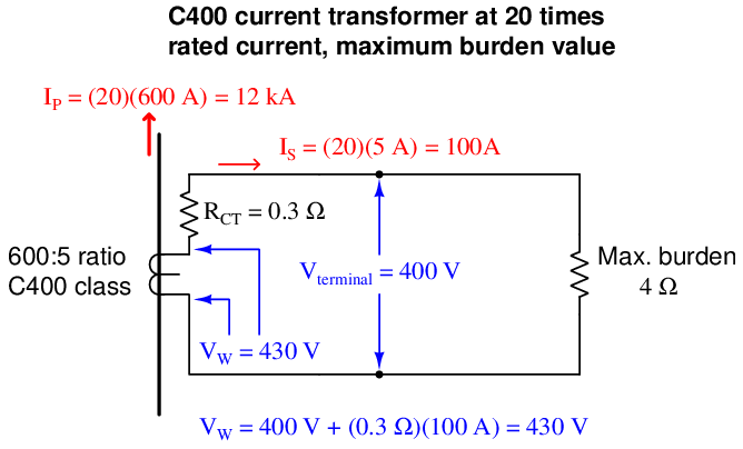
Although the CT has a C400 class rating which means 400 volts (maximum) produced at its terminals, the winding must actually be able to produce more than 400 volts in order to overcome the voltage drop of its own internal winding resistance. In this case, with a winding resistance of 0.3 ohms carrying 100 amps of current (worst-case), the winding voltage must be 430 volts in order to deliver 400 volts at the terminals. This value of 430 volts, at 60 Hz with a sinusoidal current waveform, represents the maximum amount of magnetic flux this CT’s core can handle while maintaining a current ratio within ± 10% of its 600:5 rating. Thus, 430 volts (inside the CT) is our limiting factor for the CT’s winding at any current value.
This step of calculating the CT’s maximum internal winding voltage is not merely an illustration of how a CT’s “C” class rating is defined. Rather, this is an essential step in any analysis of CT circuit burden because we must know the maximum winding potential the CT is limited to. One might be tempted to skip this step and simply use 400 volts as the maximum terminal voltage during a fault condition, but doing so will lead to minor errors in a simple case such as this, and much more significant errors in other cases where we must de-rate the CT’s winding voltage for reasons described later in this section.
Suppose this CT will be used to supply current to a protective relay presenting a purely resistive burden of 0.2 ohms. A system study reveals maximum symmetrical fault current to be 10,000 amps, which is just below the 20× rated primary current for the CT. Here is what the circuit will look like during this fault condition with the CT producing its maximum (internal) voltage of 430 volts:
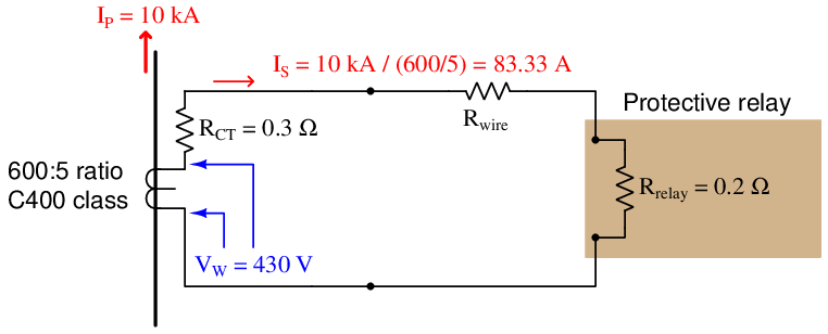
The CT’s internal voltage limit of 430 volts still holds true, because this is a function of its core’s magnetic flux capacity and not line current. With a power system fault current of 10,000 amps, this CT will only output 83.33 amps rather than the 100 amps used to define its C400 classification. The maximum total circuit resistance is easily predicted by Ohm’s Law, with 430 volts (limited by the CT’s magnetic core) pushing 83.33 amps (limited by the system fault current):

Since we know the total resistance in this series circuit is the sum of CT winding resistance, wire resistance, and relay burden, we may easily calculate maximum wire resistance by subtraction:


Thus, we are allowed to have up to 4.66 Ω of total wire resistance in this CT circuit while remaining within the CT’s ratings. Assuming the use of 12 gauge copper wire:

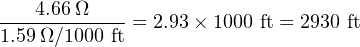
Of course, this is total conductor length, which means for a two-conductor cable between the CT and the protective relay the maximum distance will be half as much: 1465 feet.
Example: CT circuit wire sizing, with DC considered
The previous scenario assumes purely AC fault current. Real faults may contain significant DC components for short periods of time, the duration of these DC transients being related to the L R time constant of the power circuit. As previously mentioned, direct current tends to magnetize the ferrous core of a CT, predisposing it to magnetic saturation. Thus, a CT under these conditions will not be able to generate the full AC voltage possible during a controlled bench test (e.g. a C400 current transformer under these conditions will not be able to live up to its 400-volt terminal rating). A simple way to compensate for this effect is to de-rate the CT’s winding voltage by a factor equal to 1 + X R , the ratio X R being the reactance-to-resistance ratio of the power system at the point of measurement. De-rating the transformer provides a margin of safety for our calculations, anticipating that a fair amount of the CT’s magnetic core capacity may be consumed by DC magnetization during certain faults, leaving less magnetic “headroom” to generate an AC voltage.
Let’s re-do our calculations assuming the power system being protected now has an X R ratio of 14. This means our C400 current transformer (with a maximum internal winding potential of 430 volts) must be “de-rated” to a maximum winding voltage of:
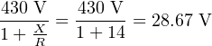
If we apply this de-rated winding voltage to the same CT circuit, we find it is insufficient to drive 83.33 amps through the relay:
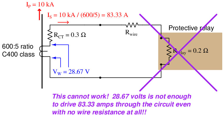
With 0.5 Ω of combined CT and relay resistance (and no wire resistance), a winding voltage of 28.67 volts could only drive 57.33 amps which is far less than we need. Clearly this CT will not be able to perform under fault conditions where DC transients push it closer to magnetic saturation.
Upgrading the CT to a different model having a higher accuracy class (C800) and a larger current step-down ratio (1200:5) will improve matters. Assuming an internal winding resistance of 0.7 ohms for this new CT, we may calculate its maximum internal winding voltage as follows: if this CT is rated to supply 800 volts at its terminals at 100 amps secondary current through 0.7 ohms of internal resistance, it must mean the CT’s secondary winding internally generates 70 volts more than the 800 volts at its terminals, or 870 volts under purely AC conditions. With our power system’s X R ratio of 14 to account for DC transients, this means we must de-rate the CT’s internal winding voltage from 870 volts to 15 times less, or 58 volts. Applying this new CT to the previous fault scenario:
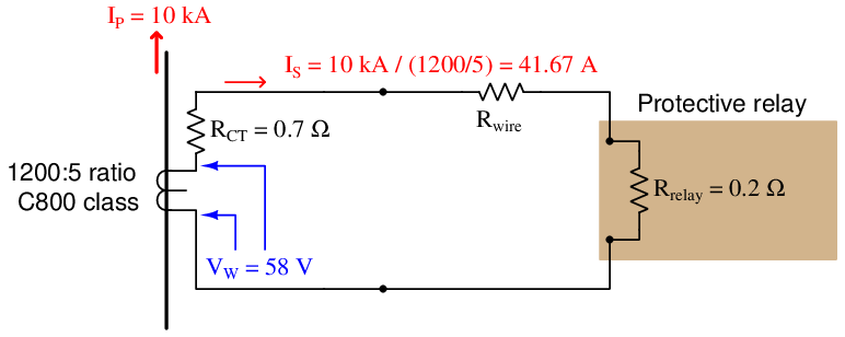
Calculating the allowable total circuit resistance given the new CT’s improved voltage:

Once again, we may calculate maximum wire resistance by subtracting all other resistances from the maximum total circuit resistance:


Thus, we are allowed to have up to 0.492 Ω of wire resistance in this circuit while remaining within the CT’s ratings. Using 10 AWG copper wire (exhibiting 1 ohm per 1000 feet), this allows us a total conductor length of 492 feet, which is 246 feet of distance between the CT terminals and the relay terminals.