
“Radio” systems use electromagnetic fields to communicate information over long distances through open space. This section explores some of the basic components common to all radio systems, as well as the mathematical analyses necessary to predict the performance of radio communication.
17.1.1 Antennas
A radio wave is a form of electromagnetic radiation, comprised of oscillating electric and magnetic fields. An antenna1 is nothing more than a conductive structure designed to emit radio waves when energized by a high-frequency electrical power source, and/or generate high-frequency electrical signals when intercepting radio waves. Three common antenna designs appear here:
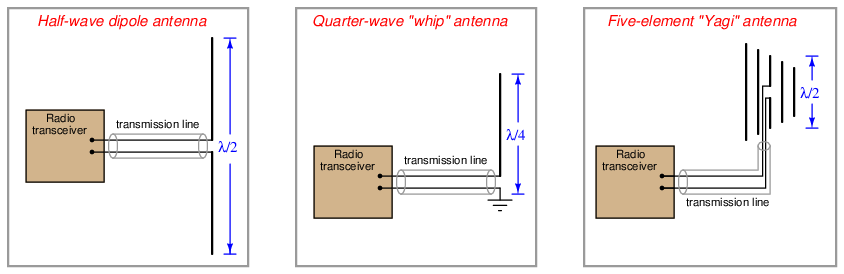
The Yagi antenna, with its “director” and “reflector” elements fore and aft of the dipole element, exhibits a high degree of directionality, whereas the dipole and “whip” antennas tend to emit and receive electromagnetic waves equally well in all directions perpendicular to their axes. Directional antennas are ideal for applications such as radar, and also in point-to-point communication applications. Omnidirectional antennas such as the dipole and whip are better suited for applications requiring equal sensitivity in multiple directions.
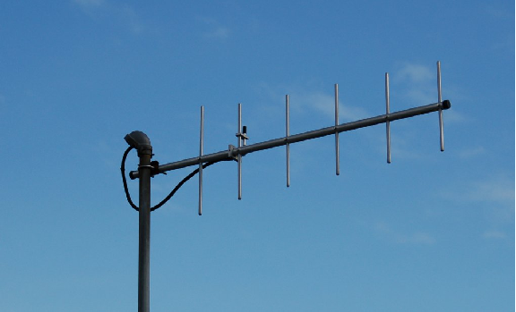
A photograph of an actual Yagi antenna used in a SCADA system appears here:
The wavelength (λ) of any wave is its propagation velocity divided by its frequency. For radio waves, the propagation velocity is the speed of light (2.99792 × 10⁸ meters per second, commonly represented as c), and the frequency is expressed in Hertz:

Antenna dimensions are related to signal wavelength because antennas work most effectively in a condition of electrical resonance. In other words, the physical size of the antenna is such that it will electrically resonate at certain frequencies: a fundamental frequency as well as the harmonics (integer-multiples) of that fundamental frequency. For this reason, antenna size is inversely proportional to signal frequency: low-frequency antennas must be large, while high-frequency antennas may be small.
For example, a quarter-wave “whip” antenna designed for a 900 MHz industrial transceiver application will be approximately2 8.3 centimeters in length. The same antenna design applied to an AM broadcast radio transmitter operating at 550 kHz would be approximately 136 meters in length!
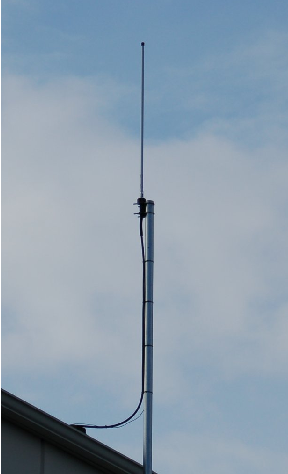
The following photograph shows a half-wave “whip” antenna, located at the roofline of a building. The additional length of this design makes it more efficient than its quarter-wave cousin. This particular antenna stands approximately one meter in length from connector to tip, yielding a full wavelength value (λ) of 2 meters, equivalent to 150 MHz:
17.1.2 Decibels
One of the mathematical tools popularly used in radio-frequency (RF) work is the common logarithm, used to express power ratios in a unit called the decibel. The basic idea of decibels is to express a comparison of two electrical powers in logarithmic terms. Every time you see the unit of “decibel” you can think: this is an expression of how much greater (or how much smaller) one power is to another. The only question is which two powers are being compared.
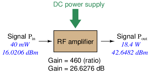
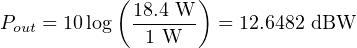
Electronic amplifiers are a type of electrical system where comparisons of power are useful. Students of electronics learn to compare the output power of an amplifier against the input power as a unitless ratio, called a gain. Take for example an electronic amplifier with a signal input of 40 milliwatts and a signal output of 18.4 watts:
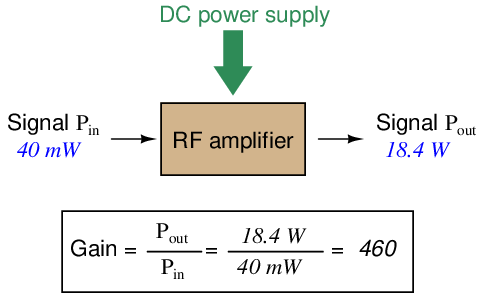
An alternative way to express the gain of this amplifier is to do so using the unit of the Bel, defined as the common logarithm of the gain ratio:
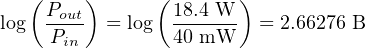
When you see an amplifier gain expressed in the unit of “Bel”, it’s really just a way of saying “The output signal coming from this amplifier is x powers of ten greater than the input signal.” An amplifier exhibiting a gain of 1 Bel outputs 10 times as much power as the input signal. An amplifier with a gain of 2 Bels boosts the input signal by a factor of 100. The amplifier shown above, with a gain of 2.66276 Bels, boosts the input signal 460-fold.
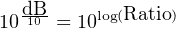
At some point in technological history it was decided that the “Bel” (B) was too large and unwieldy of a unit, and so it became common to express powers in fractions of a Bel instead: the deciBel (1 dB = 1_ 10 of a Bel). Therefore, this is the form of formula you will commonly see for expressing RF powers:
The gain of our hypothetical electronic amplifier, therefore, would be more commonly expressed as 26.6276 dB rather than 2.66276 B, although either expression is technically valid3 .
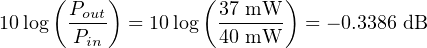
An operation students often struggle with is converting a decibel figure back into a ratio, since the concept of logarithms seems to be universally perplexing. Here I will demonstrate how to algebraically manipulate the decibel formula to solve for the power ratio given a dB figure.
First, we will begin with the decibel formula as given, solving for a value in decibels given a power ratio:

If we wish to solve for the ratio, we must “undo” all the mathematical operations surrounding that variable. One way to determine how to do this is to reverse the order of operations we would follow if we knew the ratio and were solving for the dB value. After calculating the ratio, we would then take the logarithm of that value, and then multiply that logarithm by 10: start with the ratio, then take the logarithm, then multiply last. To un-do these operations and solve for the ratio, we must un-do each of these operations in reverse order. First, we must un-do the multiplication (by dividing by 10):
Next, we must un-do the logarithm function by applying its mathematical inverse to both sides of the formula – making each expression a power of 10:

To test our algebra, we can take the previous decibel value for our hypothetical RF amplifier and see if this new formula yields the original gain ratio:


Sure enough, we arrive at the correct gain ratio of 460, starting with the decibel gain figure of 26.6276 dB.
We may also use decibels to express power losses in addition to power gains. Here, we see an example of a radio-frequency (RF) signal cable losing power along its length4 , such that the power out is less than the power in:
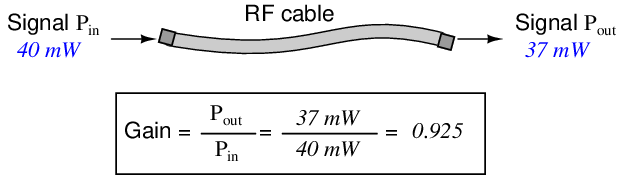
Contrasting this result against the previous result (with the amplifier) we see a very important property of decibel figures: any power gain is expressed as a positive decibel value, while any power loss is expressed as a negative decibel value. Any component outputting the exact same power as it takes in will exhibit a “gain” value of 0 dB (equivalent to a gain ratio of 1).
Remember that Bels and decibels are nothing more than logarithmic expressions of “greater than” and “less than”. Positive values represent powers that are greater while negative values represent powers that are lesser. Zero Bel or decibel values represent no change (neither gain nor loss) in power.
A couple of simple decibel values are useful to remember for approximations, where you need to quickly estimate decibel values from power ratios (or vice-versa). Each addition or subtraction of 10 dB exactly represents a 10-fold multiplication or division of power ratio: e.g. +20 dB represents a power ratio gain of 10 × 10 = 100, whereas −30 dB represents a power ratio reduction of 1 _ 10 × 1 _ 10 × 1 _ 10 = 1_ 1000. Each addition or subtraction of 3 dB approximately represents a 2-fold multiplication or division or power ratio: e.g. +6 dB is approximately equal to a power ratio gain of 2 × 2 = 4, whereas −12 dB is approximately equal to a power ratio reduction of 1 2 × 1 2 × 1 2 × 1 2 = 1 _ 16. We may combine ± 10 dB and ± 3 dB increments to come up with ratios that are products of 10 and 2: e.g. +26 dB is approximately equal to a power ratio gain of 10 × 10 × 2 × 2 = 400.
Observe what happens if we combine a “gain” component with a “loss” component and calculate the overall power out versus power in:
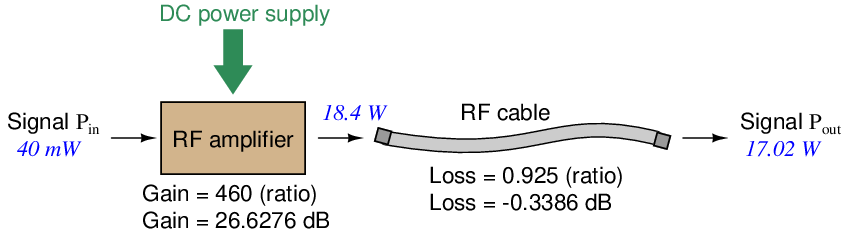
The overall gain of this RF amplifier and cable system expressed as a ratio is equal to the product of the individual component gain/loss ratios. That is, the gain ratio of the amplifier multiplied by the loss ratio of the cable yields the overall power ratio for the system:

The overall gain may be alternatively expressed as a decibel figure, in which case it is equal to the sum of the individual component decibel values. That is, the decibel gain of the amplifier added to the decibel loss of the cable yields the overall decibel figure for the system:

It is often useful to be able to estimate decibel values from power ratios and vice-versa. If we take the gain ratio of this amplifier and cable system (425.5) and round it down to 400, we may easily express this gain ratio as an expanded product of 10 and 2:

Knowing that every 10-fold multiplication of power ratio is an addition of +10 dB, and that every 2-fold multiplication of power is an addition of +3 dB, we may express the expanded product as a sum of decibel values:

Therefore, our power ratio of 425.5 is approximately equal to +26 decibels.
Decibels always represent comparisons of power, but that comparison need not always be Pout∕Pin for a system component. We may also use decibels to express an amount of power compared to some standard reference. If, for example, we wished to express the input power to our hypothetical RF amplifier (40 milliwatts) using decibels, we could do so by comparing 40 mW against a standard “reference” power of exactly 1 milliwatt. The resulting decibel figure would be written as “dBm” in honor of the 1 milliwatt reference:
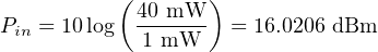
The unit of “dBm” literally means the amount of dB “greater than” 1 milliwatt. In this case, our input signal of 40 milliwatts is 16.0206 dB greater than a standard reference power of exactly 1 milliwatt. The output power of that amplifier (18.4 watts) may be expressed in dBm as well:
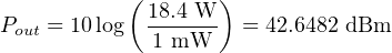
A signal power of 18.4 watts is 42.6482 dB greater than a standard reference power of exactly 1 milliwatt, and so it has a decibel value of 42.6482 dBm.
Notice how the output and input powers expressed in dBm relate to the power gain of the amplifier. Taking the input power and simply adding the amplifier’s gain factor yields the amplifier’s output power in dBm:


An electronic signal that begins 16.0206 dB greater than 1 milliwatt, when boosted by an amplifier gain of 26.6276 dB, will become 42.6482 dB greater than the original reference power of 1 milliwatt.
We may alternatively express all powers in this hypothetical amplifier in reference to a 1-watt standard power, with the resulting power expressed in units of “dBW” (decibels greater than 1 watt):
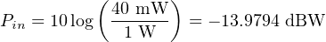
Note how the input power of 40 milliwatts equates to a negative dBW figure because 40 milliwatts is less than the 1 watt reference, and how the output power of 18.4 watts equates to a positive dBW figure because 18.4 watts is more than the 1 watt reference. A positive dB figure means “more than” while a negative dB figure means “less than.”
Note also how the output and input powers expressed in dBW still relate to the power gain of the amplifier by simple addition, just as they did when previously expressed in units of dBm. Taking the input power in units of dBW and simply adding the amplifier’s gain factor yields the amplifier’s output power in dBW:


An electronic signal that begins 13.9794 dB less than 1 watt, when boosted by an amplifier gain of 26.6276 dB, will become 12.6482 dB greater than the original reference power of 1 watt.
This is one of the major benefits of using decibels to express powers: we may very easily calculate power gains and losses by summing a string of dB figures, each dB figure representing the power gain or power loss of a different system component. Normally, any conflation of ratios involves multiplication and/or division of those ratios, but with decibels we may simply add and subtract. One of the interesting mathematical properties of logarithms is that they “transform5 ” one type of problem into a simpler type: in this case, a problem of multiplying ratios into a (simpler) problem of adding decibel figures.
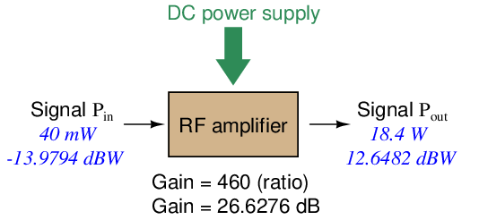
For example, we may express the power lost in an RF transmission line (two-conductor cable) in terms of decibels per foot. Most of this power loss is due to dielectric heating, as the high-frequency electric field of the RF signal causes polarized molecules in the cable insulation to vibrate and dissipate energy in the form of heat6 . The longer the cable, of course, the more power will be lost this way, all other factors being equal. A type of cable having a loss figure of −0.15 decibels per foot at a signal frequency of 2.4 GHz will suffer −15 dB over 100 feet, and −150 dB over 1000 feet. To illustrate how decibels may be used to calculate power at the end of an RF system, accounting for various gains and losses along the way using decibel figures:
17.1.3 Antenna radiation patterns
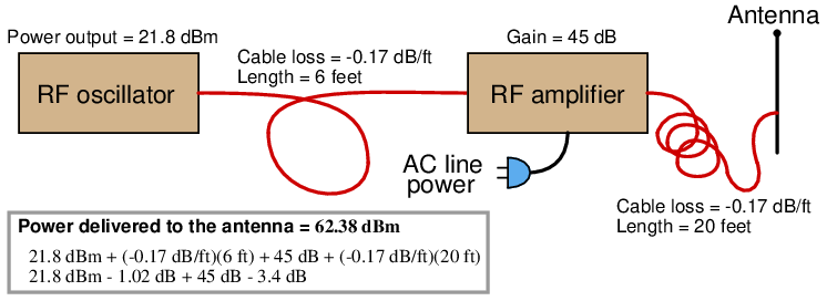
Different antenna designs are unequal with regard to how well they radiate (and receive) electromagnetic energy. Every antenna design has a pattern of radiation and sensitivity: some directions in which it is maximally effective and other directions where it is minimally effective.
Some common antenna types and radiation patterns are shown in the following illustrations, the relative radii of the shaded areas representing the degree7 of effectiveness in those directions away from or toward the antenna:
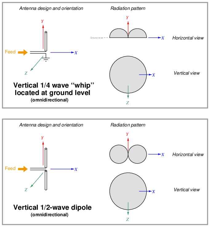
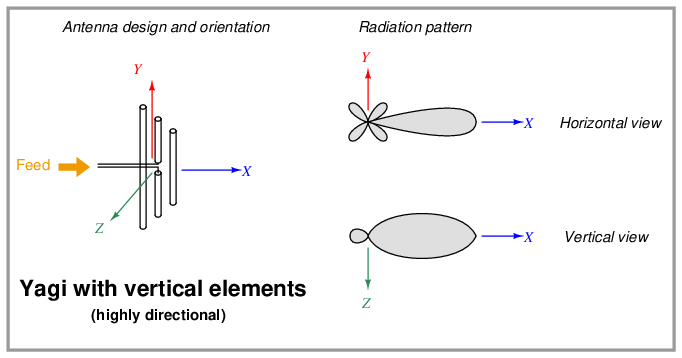
It should be noted that the radiation patterns shown here are approximate, and may modify their shapes if the antenna is operated harmonically rather than at its fundamental frequency.
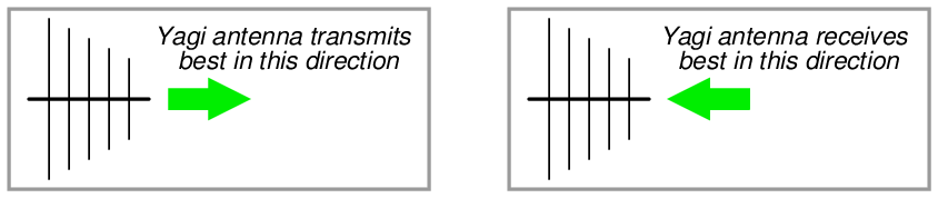
A basic principle in antenna theory called reciprocity states that the efficiency of an antenna as a radiator of electromagnetic waves mirrors its efficiency as a collector of electromagnetic waves. In other words, a good transmitting antenna will be a good receiving antenna, and an antenna having a preferred direction of radiation will likewise be maximally sensitive to electromagnetic waves approaching from that same direction. To use a Yagi as an example:
Related to reciprocity is the concept of equivalent orientation between transmitting and receiving antennas for maximum effectiveness. The electromagnetic waves emitted by a transmitting antenna are polarized in a particular orientation, with the electric and magnetic fields perpendicular to each other. The same design of antenna will be maximally receptive to those waves if its elements are similarly oriented. A simple rule to follow is that antenna pairs should always be parallel to each other in order to maximize reception, in order that the electric and magnetic fields emanating from the wires of the transmitting antenna will “link” properly with the wires of the receiving antenna(s). If the goal is optimum communication in any direction (omnidirectionality), dipole and whip antennas should be arranged vertically so that all antenna conductors will be parallel to each other regardless of their geographic location.
Yagi antenna pairs may be horizontally or vertically oriented, so long as the transmitting and receiving Yagis are both mounted with the same polarization and face each other. In industrial SCADA radio applications, Yagi antennas are generally oriented with the dipole wires vertical, so that they may be used in conjunction with omnidirectional whip or dipole antennas. An illustration of such use is shown here, with multiple “Remote Terminal Unit” (RTU) transceivers communicating with a central “Master Terminal Unit” (MTU) transceiver:
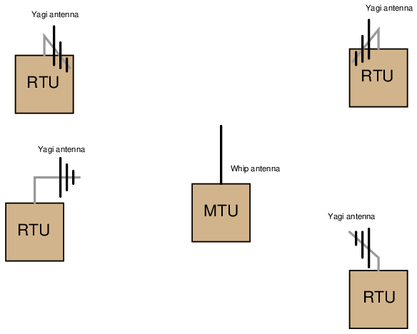
Here, all the Yagi antennas on the RTUs are vertically oriented, so that they will match the polarization of the MTU’s whip antenna. The Yagi antennas all face in the direction of the MTU for optimum sensitivity. The MTU – which must broadcast to and receive from all the RTUs – really needs an omnidirectional antenna. The RTUs – which need only communicate with the one MTU and not with each other – work best with highly directional antennas.
If the MTU were equipped with a Yagi antenna instead of a whip, it would only communicate well with one of the RTUs, and perhaps not at all with some of the others. If all RTUs were equipped with whip antennas instead of Yagis, they would not be as receptive to the MTU’s broadcasts (lower gain), and each RTU would require greater transmitter power to transmit effectively to the MTU.
Another important principle to employ when locating any antenna is to keep it far away from any conductive surfaces or objects, including soil. Proximity to any conductive mass distorts an antenna’s radiation pattern, which in turn affects how well it can transmit and receive in certain directions. If there is any consistent rule to follow when setting up antennas for maximum performance, it is this: position them as high as possible and as far away from interfering objects as possible!
17.1.4 Antenna gain calculations
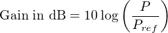
A common way to express the maximal effectiveness of any antenna design is as a ratio compared to some idealized form of antenna with a more uniform radiation pattern. As with most ratio measurements in radio technology, the standard unit for antenna gain is the decibel (dB), related to a ratio of powers as follows:
The most common reference standard used to calculate antenna gain is a purely theoretical device called an isotropic antenna. This is an ideally omnidirectional antenna having a perfectly spherical radiation pattern:
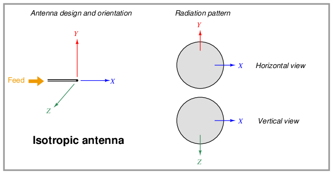
If a directional antenna such as a Yagi radiates (and/or receives) 20 times as much power in its most sensitive direction as an isotropic antenna, it is said to have a power gain of 13.01 dBi (13.01 decibels more than an isotropic). An alternative “reference” for comparison is a half-wave dipole antenna. Decibel comparisons against a dipole are abbreviated dBd. The assumption of an isotropic antenna as the reference is so common in radio engineering, though, you often see antenna gains expressed simply in units of dB. The assumption of isotropic reference (dBi) for antenna gain expressions is analogous to the assumption of “RMS” measurements in AC circuits rather than “peak” or “peak-to-peak”: if you see an AC voltage expressed without any qualifier (e.g. “117 volts AC”), it is generally assumed to be an RMS measurement.
Whip antennas typically exhibit an optimal gain of 6 dBi (6 dB being approximately equal to a 4-fold magnification compared to an isotropic antenna), while Yagis may achieve up to 15 dBi (approximately equal to a 32-fold magnification). Parabolic “dish” antenna designs such as those used in microwave communication systems may achieve gains as high as 30 dBi (≈ 1000-fold magnification). Since antenna gain is not a real amplification of power – this being impossible according to the Law of Energy Conservation – greater antenna gain is achieved only by greater focus of the radiation pattern in a particular direction.
The concept of antenna gain is very easy to mis-comprehend, since it is tempting to think of any type of gain as being a true increase in power. Antenna gain is really nothing more than a way to express how concentrated the RF energy of a radiating8 antenna is in one direction compared to a truly omnidirectional antenna. An analogy to antenna gain is how a horn-style loudspeaker focuses its audio energy more than a loudspeaker lacking a horn. The horn-shaped speaker sounds louder than the horn-less speaker (in one direction only) because its audio energy is more focused. The two speakers may be receiving the exact same amount of electrical energy to produce sound, but the more directional of the two speakers will be more efficient transmitting sound in one direction than the other. Likewise, a horn-shaped microphone will have greater sensitivity in one direction than a comparable “omni” microphone designed to receive sound equally well from all directions. Connected to a recording device, the directional microphone seems to present a “gain” by sending a stronger signal to the recorder than the omnidirectional microphone is able to send, in that one direction.
The flip-side of high-gain antennas, loudspeakers, and microphones is how poorly they perform in directions other than their preferred direction. Any transmitting or receiving structure exhibiting a “gain” due to its focused radiation pattern must likewise exhibit a “loss” in performance when tested in directions other than its direction of focus. Referring back to directional radio antennas again, a Yagi with an advertised gain of 15 dBi (in its “preferred” direction) will exhibit a strong negative gain in the rearward direction where its ability to radiate and receive is almost non-existent.
If even more signal gain is necessary than what may be achieved by narrower radiation focus, an actual electronic amplifier may be added to an antenna assembly to boost the RF power sent to or received from the antenna. This is common for satellite antenna arrays, where the RF amplifier is often located right at the focal point of the parabolic dish. Satellite communication requires very high transmitter and receiver gains, due to inevitable signal weakening over the extremely long distances between a ground-based antenna and a satellite antenna in geosynchronous orbit around the Earth.
17.1.5 Effective radiated power
When determining the effectiveness of a radio system, one must include losses in cables, connectors, lightning arrestors, and other elements in the signal path in addition to the antenna itself. A commonly accepted way to quantify this effectiveness is to rate a radio system against a standard reference consisting of an ideal dipole antenna connected to a 1 milliwatt transmitter with no losses. Typically expressed in units of decibels, this is called the Effective Radiated Power, or ERP. If the ideal antenna model is isotropic instead of a dipole, then the calculation result is called the Effective Isotropic Radiated Power, or EIRP.
Let us consider the following example, where a 2.4 GHz radio transceiver outputs 250 milliwatts9 of radio-frequency (RF) power to a Yagi antenna through a type LMR 195 coaxial cable 12 feet in length. A lightning arrestor with 0.5 dB loss is also part of the cable system. We will assume an antenna gain of 9 dBi for the Yagi and a loss of 0.19 dB per foot for the LMR 195 cable:
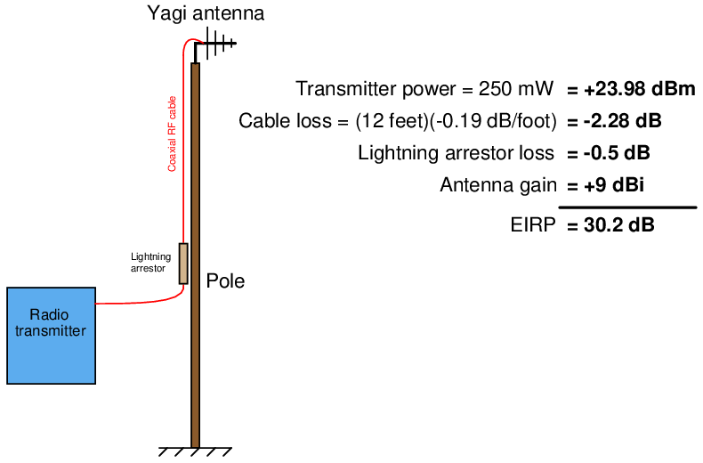
The EIRP for this radio system is 30.2 dB: the sum of all gains and losses expressed in decibels. This means our Yagi antenna will radiate 30.2 dB (1047 times) more RF power in its most effective direction than an isotropic antenna would radiate in the same direction powered by a 1 milliwatt transmitter. Note that if our hypothetical radio system also included an RF amplifier between the transceiver and the antenna, its gain would have to be included in the EIRP calculation as well.
A practical application of EIRP is how the Federal Communications Commission (FCC) sets limits on radio transmitters within the United States. Not only is gross transmitter power limited by law within certain frequency ranges, but also the EIRP of a transmitting station. This makes sense, since a more directional transmitting antenna (i.e. one having a greater gain value) will make it appear as though the transmitter is more powerful than it would be radiating from a less-directional antenna. If FCC limits were based strictly on transmitter power output rather than EIRP, it might still be possible for an otherwise power-compliant transmitting station to generate excessive interference through the use of a highly directional antenna. This is why it is illegal, for example, to connect a large antenna to a low-power transmitting device such as a two-way (“walkie-talkie”) radio unit: the two-way radio unit may be operated license-free only because its EIRP is low enough not to cause interference with other radio systems. If someone were to connect a more efficient antenna to this same two-way radio, its effective radiated power may increase to unacceptable levels (according to the FCC) even though the raw power output by the transmitter circuitry has not been boosted.
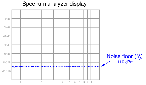
17.1.6 RF link budget
Electromagnetic radiation is used as a medium to convey information, to “link” data from one physical location to another. In order for this to work, the amount of signal loss between transmitter and receiver must be small enough that the signal does not become lost in radio-frequency “noise” originating from external sources and from within the radio receiver itself. We may express radio-frequency (RF) power in terms of its comparison to 1 milliwatt: 0 dBm being 1 milliwatt, 3.01 dBm being 2 milliwatts, 20 dBm being 100 milliwatts, etc. We may use dBm as an absolute measurement scale for transmitted and received signal strengths, as well as for expressing how much ambient RF noise is present (called the “noise floor” for its appearance at the bottom of a spectrum analyzer display). We may use plain dB to express relative gains and losses along the signal path.
The basic idea behind an “RF link budget” is to add all gains and losses in an RF system – from transmitter to receiver with all intermediate elements accounted for – to ensure there is a large enough difference between signal and noise to ensure good data communication integrity. If we account all gains as positive decibel values and all losses as negative decibel values, the signal power at the receiver will be the simple sum of all the gains and losses:

Where,
Prx = Signal power delivered to receiver input (dBm)
Ptx = Transmitter output signal power (dBm)
Gtotal = Sum of all gains (amplifiers, antenna directionality, etc.), a positive dB value
Ltotal = Sum of all losses (cables, filters, path loss, fade, etc.), a negative dB value
This formula tells us how much signal power will be available at the radio receiver, but usually the purpose of calculating a link budget is to determine how much radio transmitter power will be necessary in order to have adequate signal strength at the receiver. More transmitter power adds expense, not only due to transmitter hardware cost but also to FCC licenses that are required if certain power limitations are exceeded. Excessive transmitter power may also create interference problems with other radio and electronic systems. Suffice it to say we wish to limit transmitter power to the minimum practical value.
In order for a radio receiver to reliably detect an incoming signal, that signal must be sufficiently greater than the ambient RF noise. All masses at temperatures above absolute zero radiate electromagnetic energy, with some of that energy falling within the RF spectrum. This noise floor value may be calculated10 or empirically measured using an RF spectrum analyzer as shown in this simulated illustration:
On top of the ambient noise, we also have the noise figure of the receiver itself (Nrx): noise created by the internal circuitry of the radio receiver. Thus, the minimum signal power necessary for the receiver to operate reliably (Prx(min)) is equal to the decibel sum of the noise floor and the noise figure, by a margin called the minimum signal-to-noise ratio:

Where,
Prx(min) = Minimum necessary signal power at the receiver input (dBm)
Nf = Noise floor value (dBm)
Nrx = Noise figure of radio receiver (dB)
S = Desired signal-to-noise ratio margin (dB)
Substituting this decibel sum into our original RF link budget formula and solving for the minimum necessary transmitter power output (Ptx(min)), we get the following result:

It is common for radio receiver manufacturers to aggregate the noise floor, noise figure, and a reasonable signal-to-noise ratio into a single parameter called receiver sensitivity. The “sensitivity” of a radio receiver unit is the minimum amount of signal power (usually expressed in dBm) necessary at the input connector for reliable operation despite the inevitable presence of noise. If we simply express receiver sensitivity as Prx(min) and substitute this term for the sum of noise floor, noise figure, and signal-to-noise margin (Nf + Nrx + S) in the last formula, we see that the difference in receiver sensitivity (expressed in absolute decibels) and the sum of any gains and losses in the link (also expressed in decibels) tells us the minimum transmitter power required:

Where,
Ptx(min) = Minimum necessary transmitter output signal power, in dBm
Prx(min) = Receiver sensitivity (minimum necessary received signal power), in dBm
Gtotal = Sum of all gains (amplifiers, antenna directionality, etc.), a positive dB value
Ltotal = Sum of all losses (cables, filters, path loss, fade, etc.), a negative dB value
For digital radio receivers, sensitivity is a function of error rate: the fewer errors desired, the more signal power required. To give a practical example, one modern 900 MHz radio transceiver has a specified sensitivity of −110 dBm at a bit error rate (BER) of 10−4 bits (one error for every 104 bits received) and a sensitivity of −108 dBm at a BER of 10−6 bits. This relationship between signal power and error rate should make intuitive sense: the more powerful the signal compared to any background noise, the more reliably it will be received; the weaker the signal, the more it will become corrupted by noise and therefore the more errors we would expect to see over time.
Among the losses encompassed in Ltotal are path loss and fade. Path loss is the natural loss of signal strength with increasing distance from the radiation source. As electromagnetic waves propagate outward through space, they inevitably spread. The degradation in signal strength with increasing distance follows the inverse square law11 , where power decreases with the square of distance. Thus, doubling the distance from transmitting antenna to receiving antenna attenuates the signal by a factor of four ( 1_ 22 , or −6.02 dB). Tripling the distance from transmitting antenna to receiving antenna attenuates the signal by a factor of nine ( 1_ 32 , or −9.54 dB).
Path loss for free-space conditions is a rather simple function of distance and wavelength:
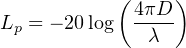
Where,
Lp = Path loss, a negative dB value
D = Distance between transmitting and receiving antennas
λ = Wavelength of transmitted RF field, in same physical unit as D
It should be emphasized that this simple path loss formula only applies to completely clear, empty space where the only mechanism of signal attenuation is the natural spreading of radio waves as they radiate away from the transmitting antenna. Path loss will be significantly greater if any objects or other obstructions lie between the transmitting and receiving antennas.
This same spreading effect also accounts for “fade,” where radio waves taking different paths deconstructively interfere (e.g. waves reflected off lateral objects reaching the receiving antenna out-of-phase with the straight-path waves), resulting in attenuated signal strengths in some places (but not in all). You may have personally experienced fade while driving a vehicle over long distances and listening to an analog (AM or FM) radio: sometimes a particular radio station’s signal will “fade out” as you drive and then “fade in” again while driving in the same direction, for no obvious reason (e.g. no immediate obstructions to the signal). This is due to radio waves from the station emanating in all directions, then reflecting off of large objects and/or ionized regions high in the earth’s atmosphere. There will inevitably be locations around that station where the incident wave from the transmitting antenna destructively interferes with those reflected waves, the result being regions of “dead” space where the signal is much weaker than one would expect from path loss alone.
Fade is a more difficult factor to predict than path loss, and so generally radio system designers include an adequate margin12 to account for the effects of fade. This fade margin is typically 20 dB to 30 dB, although it can be greater in scenarios where there are many signal paths due to reflections.
To illustrate, we will calculate the RF link budget for a 900 MHz radio transmitter/receiver pair directionally oriented toward each other with Yagi antennas. All sources of signal gain and loss will be accounted for, including the “path loss” of the RF energy as it travels through open air. The gains and losses of all elements are shown in the following illustration:
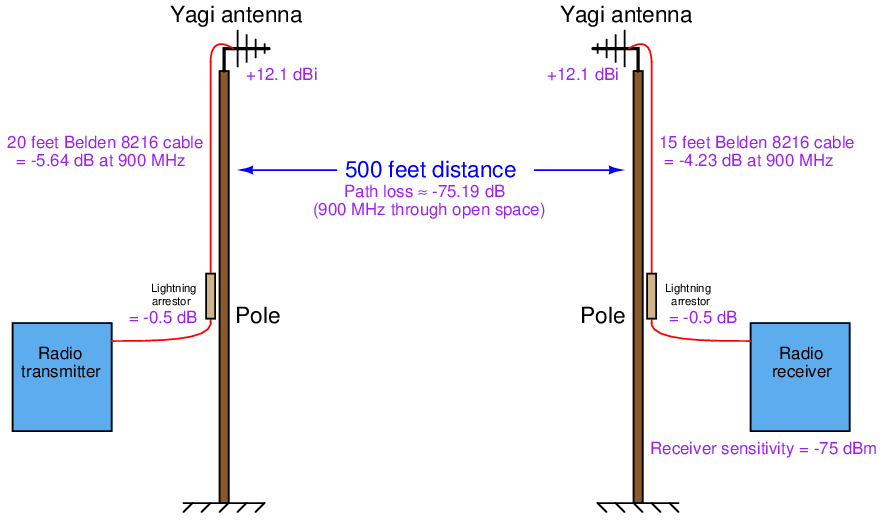
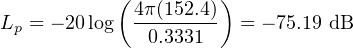
The path loss value shown in the illustration is a calculated function of the 900 MHz wavelength (λ = c f = 0.3331 meters) and the distance between antennas (500 feet = 152.4 meters), assuming a completely obstruction-free path between antennas:
According to the receiver manufacturer’s specifications, the receiver in this system has a sensitivity of −75 dBm, which means our transmitter must be powerful enough to deliver an RF signal at least as strong as −75 dBm at the receiver’s input connector in order to reliably communicate data. Inserting this receiver sensitivity figure into our RF link budget formula:


Now we need to tally all the gains and losses between the transmitter and the receiver. We will use a value of −20 dB for fade margin (i.e. our budget will leave room for up to 20 dB of power loss due to the effects of fade):
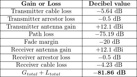
Inserting the decibel sum of all gains and losses into our RF link budget formula:


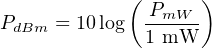
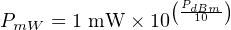
Converting a dBm value into milliwatts of RF power means we must manipulate the dBm power formula to solve for PmW:

At this point we would do well to take stock of the assumptions intrinsic to this calculation. Power gains and losses inherent to the components (cables, arrestors, antennas) are quite certain because these are tested components, so we need not worry about these figures too much. What we know the least about are the environmental factors: noise floor can change, path loss will differ from our calculation if there is any obstruction near the signal path or under certain weather conditions (e.g. rain or snow dissipating RF energy), and fade loss is known to change dynamically as moving objects (people, vehicles) pass anywhere between the transmitter or receiver antennas. Our RF link budget calculation is really only an estimate of the transmitter power needed to get the job done.
How then do we improve our odds of building a reliable system? One way is to over-build it by equipping the transmitter with more power than the most pessimistic link budget predicts. However, this can cause other problems such as interference with nearby electronic systems if we are not careful. A preferable method is to conduct a site test where the real equipment is set up in the field and tested to ensure adequate received signal strength.
17.1.7 Link budget graph
Many of the concepts previously explored may be represented in a single graph13 , showing RF signal strength as a function of physical position within the RF link (from transmitter to receiver). The horizontal axis of this graph represents the position along the link path from transmitter to receiver, while the vertical axis represents RF signal strength in dBm:
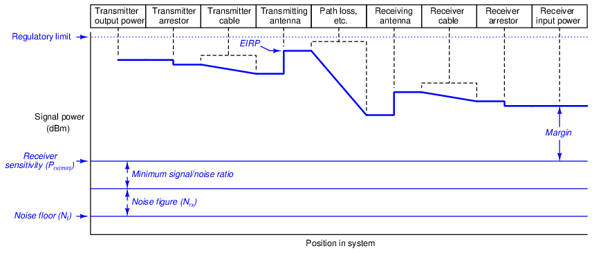
At the very bottom of this graph we see the noise floor, representing natural RF noise that is unavoidable. Above that we see the added noise figure and signal/noise ratios summing up to a higher line representing the receiver’s sensitivity, which is the minimum amount of signal power it must receive in order to reliably function.
Near the top of this graph we see a series of thicker line segments representing the various losses and gains within the system. Single-point losses such as lightning arrestors appear as vertical downward steps, while progressive losses such as cables and path loss appear as downward slopes. Single-point gains such as antennas appear as vertical upward steps. Note where EIRP appears on this graph: the amount of signal power at the transmitting antenna’s output, factoring in the antenna’s gain as well as any losses between the transmitter and the transmitting antenna. As previously mentioned, the Federal Communications Commission (FCC) sets regulatory limits for EIRP in the United States, because if only the transmitter’s output power were regulated, it would be possible to thwart that limit using high-gain antennas.
At the far right-hand end of the graph, we see the difference between the receiver’s input signal power and the receiver’s sensitivity as a margin for the link budget. This margin must exist in order to grant the system tolerance to unexpected power losses such as those resulting from inclement weather, interference from objects within the link path, cable deterioration, coupling corrosion, increases in noise floor, etc.
17.1.8 Fresnel zones
One of the many factors affecting RF link power transfer from transmitter to receiver is the openness of the signal path between the transmitting and receiving antennas. As shown in the previous subsection, path loss is relatively simple to calculate given the assumption of totally empty space between the two antennas. With no obstacles in between, path loss is simply a consequence of wave dispersion (spreading). Unless we are calculating an RF link budget between two airplanes or two spacecraft, though, there really is no such thing as totally empty space between the transmitting and receiving antennas. Buildings, trees, vehicles, and even the ground are all objects potentially disrupting what would otherwise be completely open space between transmitter and receiver.
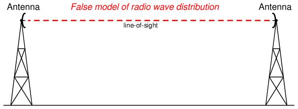
A common expression in microwave radio communication is line-of-sight, or LoS. The very wording of this phrase evokes an image of being able to see a straight path between transmitting and receiving antennas. Obviously, if one does not have a clear line-of-sight path between antennas, the signal path loss will definitely be more severe than through open space. However, a common error is in thinking that the mere existence of an unobstructed straight line between antennas is all that is needed for unhindered communication, when in fact nothing could be further from the truth:
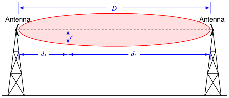
In fact, the free space necessary to convey energy in electromagnetic wave form takes on the form of football-shaped zones: the first one solid followed by annular (hollow) zones concentrically surrounding the first. These elliptical volumes are called Fresnel zones:
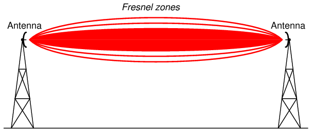
The precise shapes of these Fresnel zones are a function of wavelength and distance between antennas, not the size or configurations of the antennas themselves. In other words, you cannot change the Fresnel zone sizes or shapes by merely altering antenna types. This is because the Fresnel zones do not actually map the distribution of electromagnetic fields, but rather map the free space we need to keep clear between antennas14 .
If any object protrudes at all into any Fresnel zone, it diminishes the signal power communicated between the two antennas. In microwave communication (GHz frequency range), the inner-most Fresnel zone carries most of the power, and is therefore the most important from the perspective of interference. Keeping the inner-most Fresnel zone absolutely clear of interference is essential for maintaining ideal path-loss characteristics (equivalent to open-space). A common rule followed by microwave system designers is to try to maintain an inner Fresnel zone that is at least 60% free of obstruction.
In order to design a system with this goal in mind, we need to have some way of calculating the width of that Fresnel zone. Fortunately, this is easily done with the following formula:
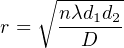
Where,
r = Radius of Fresnel zone at the point of interest
n = Fresnel zone number (an integer value, with 1 representing the first zone)
d1 = Distance between one antenna and the point of interest
d2 = Distance between the other antenna and the point of interest
D = Distance between both antennas
λ = Wavelength of transmitted RF field, in same physical unit as D, d1, and d2
Note: the units of measurement in this formula may be any unit of length, so long as they are all the same unit.
To illustrate by example, let us calculate the radius of the first Fresnel zone for two microwave antennas operating at 2.4 GHz, separated by one mile (1.609 km), at the widest portion of that zone. The wavelength of a 2.4 GHz signal is 0.1249 meters, from the formula λ = c f . Distances d1 and d2 will both be equal to one-half of the total distance, since the widest portion of the Fresnel zone will be exactly at its mid-point between the two antennas (d1 = d2 = 804.7 meters). Here, we solve for r as follows:

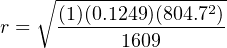

Consider for a moment the significance of this dimension. At the very least, it means the antennas must be mounted this high off the ground in order to avoid having the most important Fresnel zone contact the earth itself (assuming level terrain), not to mention any objects above ground level such as buildings, vehicles, or trees between the two antennas. Consider also that the Fresnel zone is football-shaped, and therefore this 7.089 meter radius extends horizontally from the centerline connecting both antennas as well as vertically. This means that in order for this Fresnel zone to be untouched, there must be a clear path 14.18 meters wide in addition to the antennas being at least 7.089 meters off the ground! If we were to consider a 900 MHz signal – another common frequency for industrial wireless devices – the minimum height above ground would be 11.58 meters, and the minimum clear path width 23.16 meters!
As you can see, “line of sight” is not as simple as it may first appear.