
In the United States, the most common language used to program PLCs is Ladder Diagram (LD), also known as Relay Ladder Logic (RLL). This is a graphical language showing the logical relationships between inputs and outputs as though they were contacts and coils in a hard-wired electromechanical relay circuit. This language was invented for the express purpose of making PLC programming feel “natural” to electricians familiar with relay-based logic and control circuits. While Ladder Diagram programming has many shortcomings, it remains extremely popular and so will be the primary focus of this chapter.
Every Ladder Diagram program is arranged to resemble an electrical diagram, making this a graphical (rather than text-based) programming language. Ladder diagrams are to be thought of as virtual circuits, where virtual “power” flows through virtual “contacts” (when closed) to energize virtual “relay coils” to perform logical functions. None of the contacts or coils seen in a Ladder Diagram PLC program are real; rather, they act on bits in the PLC’s memory, the logical inter-relationships between those bits expressed in the form of a diagram resembling a circuit.
The following computer screenshot shows a typical Ladder Diagram program16 being edited on a personal computer:
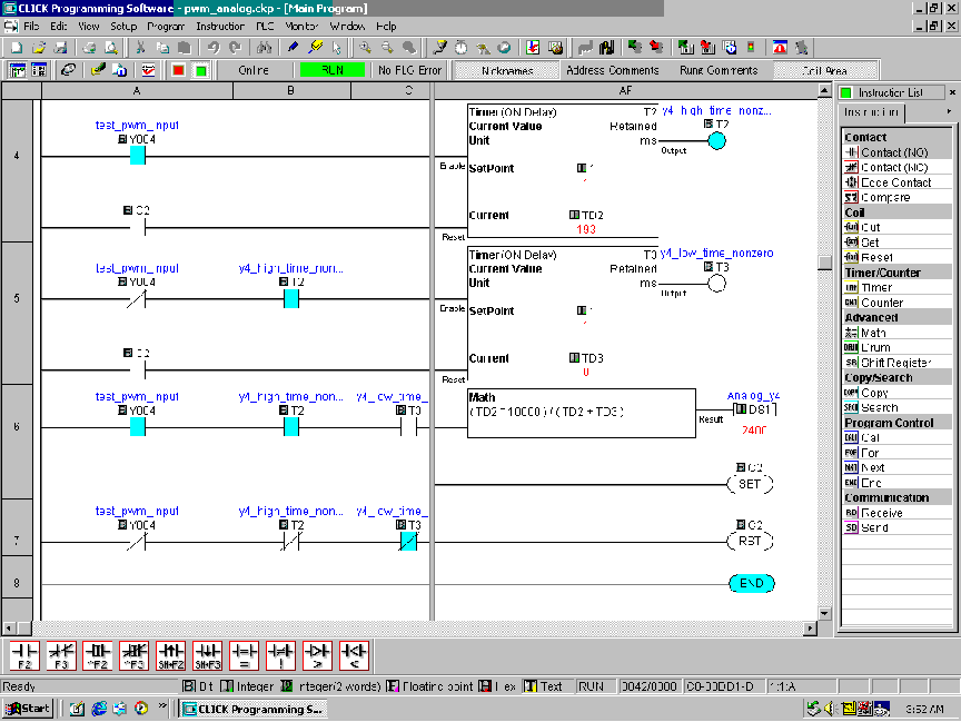
Contacts appear just as they would in an electrical relay logic diagram – as short vertical line segments separated by a horizontal space. Normally-open contacts are empty within the space between the line segments, while normally-closed contacts have a diagonal line crossing through that space. Coils are somewhat different, appearing as either circles or pairs of parentheses. Other instructions appear as rectangular boxes.
Each horizontal line is referred to as a rung, just as each horizontal step on a stepladder is called a “rung.” A common feature among Ladder Diagram program editors, as seen on this screenshot, is the ability to color-highlight those virtual “components” in the virtual “circuit” ready to “conduct” virtual “power.” In this particular editor, the color used to indicate “conduction” is light blue. Another form of status indication seen in this PLC program is the values of certain variables in the PLC’s memory, shown in red text.
For example, you can see coil T2 energized at the upper-right corner of the screen (filled with light blue coloring), while coil T3 is not. Correspondingly, each normally-open T2 contact appears colored, indicating its “closed” status, while each normally-closed T2 contact is uncolored. By contrast, each normally-open T3 contact is uncolored (since coil T3 is unpowered) while each normally-closed T3 contact is shown colored to indicate its conductive status. Likewise, the current count values of timers T2 and T3 are shown as 193 and 0, respectively. The output value of the math instruction box happens to be 2400, also shown in red text.
Color-highlighting of Ladder Diagram components only works, of course, when the computer running the program editing software is connected to the PLC and the PLC is in the “run” mode (and the “show status” feature of the editing software is enabled). Otherwise, the Ladder Diagram is nothing more than black symbols on a white background. Not only is status highlighting very useful in de-bugging PLC programs, but it also serves an invaluable diagnostic purpose when a technician analyzes a PLC program to check the status of real-world input and output devices connected to the PLC. This is especially true when the program’s status is viewed remotely over a computer network, allowing maintenance staff to investigate system problems without even being near the PLC!
12.4.1 Contacts and coils
The most elementary objects in Ladder Diagram programming are contacts and coils, intended to mimic the contacts and coils of electromechanical relays. Contacts and coils are discrete programming elements, dealing with Boolean (1 and 0; on and off; true and false) variable states. Each contact in a Ladder Diagram PLC program represents the reading of a single bit in memory, while each coil represents the writing of a single bit in memory.
Discrete input signals to the PLC from real-world switches are read by a Ladder Diagram program by contacts referenced to those input channels. In legacy PLC systems, each discrete input channel has a specific address which must be applied to the contact(s) within that program. In modern PLC systems, each discrete input channel has a tag name created by the programmer which is applied to the contact(s) within the program. Similarly, discrete output channels – referenced by coil symbols in the Ladder Diagram – must also bear some form of address or tag name label.
To illustrate, we will imagine the construction and programming of a redundant flame-sensing system to monitor the status of a burner flame using three sensors. The purpose of this system will be to indicate a “lit” burner if at least two out of the three sensors indicate flame. If only one sensor indicates flame (or if no sensors indicate flame), the system will declare the burner to be un-lit. The burner’s status will be visibly indicated by a lamp that human operators can readily see inside the control room area.
Our system’s wiring is shown in the following diagram:
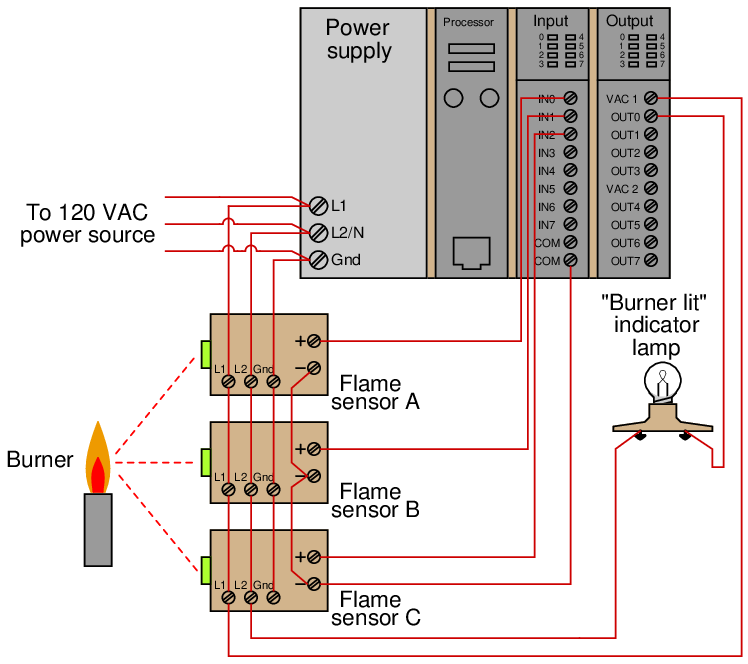
Each flame sensor outputs a DC voltage signal indicating the detection of flame at the burner, either on (24 volts DC) or off (0 volts DC). These three discrete DC voltage signals are sensed by the first three channels of the PLC’s discrete input card. The indicator lamp is a 120 volt light bulb, and so must be powered by an AC discrete output card, shown here in the PLC’s last slot.
To make the ladder program more readable, we will assign tag names (symbolic addresses) to each input and output bit in the PLC, describing its real-world device in an easily-interpreted format17 . We will tag the first three discrete input channels as IN_sensor_A, IN_sensor_B, and IN_sensor_C, and the output as OUT_burner_lit.
A ladder program to determine if at least two out of the three sensors detect flame is shown here, with the tag names referencing each contact and coil:
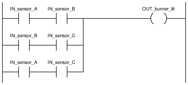
Series-connected contacts in a Ladder Diagram perform the logical AND function, while parallel contacts perform the logical OR function. Thus, this two-out-of-three flame-sensing program could be verbally described as:

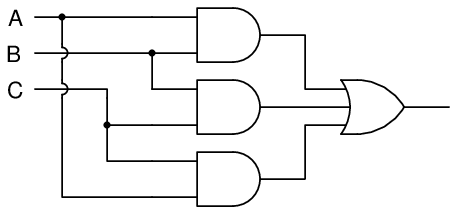
An alternate way to express this is to use the notation of Boolean algebra, where multiplication represents the AND function and addition represents the OR function:

Yet another way to represent this logical relationship is to use logic gate symbols:
To illustrate how this program would work, we will consider a case where flame sensors B and C detect flame, but sensor A does not18 . This represents a two-out-of-three-good condition, and so we would expect the PLC to turn on the “Burner lit” indicator light as programmed. From the perspective of the PLC’s rack, we would see the indicator LEDs for sensors B and C lit up on the discrete input card, as well as the indicator LED for the lamp’s output channel:
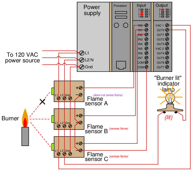
Those two energized input channels “set” bits (1 status) in the PLC’s memory representing the status of flame sensors B and C. Flame sensor A’s bit will be “clear” (0 status) because its corresponding input channel is de-energized. The fact that the output channel LED is energized (and the “Burner lit” indicator lamp is energized) tells us the PLC program has “set” that corresponding bit in the PLC’s output memory register to a “1” state.
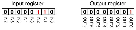
A display of input and output register bits shows the “set” and “reset” states for the PLC at this moment in time:
Examining the Ladder Diagram program with status indication enabled, we see how only the middle contact pair is passing “virtual power” to the output coil:
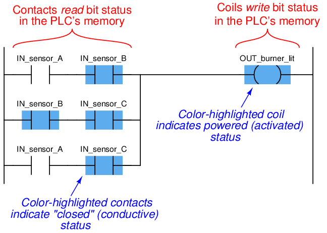
Recall that the purpose of a contact in a PLC program is to read the status of a bit in the PLC’s memory. These six “virtual contacts” read the three input bits corresponding to the three flame sensors. Each normally-open “contact” will “close” when its corresponding bit has a value of 1, and will “open” (go to its normal state) when its corresponding bit has a value of 0. Thus, we see here that the two contacts corresponding to sensor A appear without highlighting (representing no “conductivity” in the virtual relay circuit) because the bit for that input is reset (0). The two contacts corresponding to sensor B and the two contacts corresponding to sensor C all appear highlighted (representing “conductivity” in the virtual circuit) because their bits are both set (1).
Recall also that the purpose of a coil in a PLC program is to write the status of a bit in the PLC’s memory. Here, the “energized” coil sets the bit for the PLC output 0 to a “1” state, thus activating the real-world output and sending electrical power to the “Burner lit” lamp.
Note that the color highlighting does not indicate a virtual contact is conducting virtual power, but merely that it is able to conduct power. Color highlighting around a virtual coil, however, does indicate the presence of virtual “power” at that coil.
Contacts and relays are not just useful for implementing simple logic functions, but they may also perform latching functions as well. A very common application of this in industrial PLC systems is a latching start/stop program for controlling electric motors by means of momentary-contact pushbutton switches. As before, this functionality will be illustrated by means of an hypothetical example circuit and program:
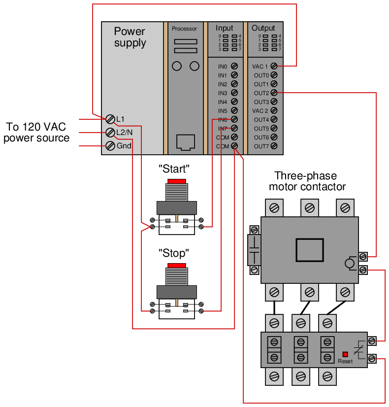
In this system, two pushbutton switches are connected to discrete inputs on a PLC, and the PLC in turn energizes the coil of a motor contactor relay by means of one of its discrete outputs19 . An overload contact is wired directly in series with the contactor coil to provide motor overcurrent protection, even in the event of a PLC failure where the discrete output channel remains energized20 .
The ladder program for this motor control system would look like this:
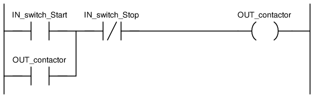
Pressing the “Start” pushbutton energizes discrete input channel 6 on the PLC, which “closes” the virtual contact in the PLC program labeled IN_switch_Start. The normally-closed virtual contact for input channel 7 (the “Stop” pushbutton) is already closed by default when the “Stop” button is not being pressed, and so the virtual coil will receive “power” when the “Start” pushbutton is pressed and the “Stop” pushbutton is not.
Note the seal-in contact bearing the exact same label as the coil: OUT_contactor. At first it may seem strange to have both a contact and a coil in a PLC program labeled identically21 , since contacts are most commonly associated with inputs and coils with outputs, but this makes perfect sense if you realize the true meaning of contacts and coils in a PLC program: as read and write operations on bits in the PLC’s memory. The coil labeled OUT_contactor writes the status of that bit, while the contact labeled OUT_contactor reads the status of that same bit. The purpose of this contact, of course, is to latch the motor in the “on” state after a human operator has released his or her finger from the “Start” pushbutton.
This programming technique is known as feedback, where an output variable of a function (in this case, the feedback variable is OUT_contactor) is also an input to that same function. The path of feedback is implicit rather than explicit in Ladder Diagram programming, with the only indication of feedback being the common name shared by coil and contact. Other graphical programming languages (such as Function Block) have the ability to show feedback paths as connecting lines between function outputs and inputs, but this capacity does not exist in Ladder Diagram.
A step-by-step sequence showing the operation and status of this simple program illustrates how the seal-in contact functions, through a start-up and shut-down cycle of the motor:
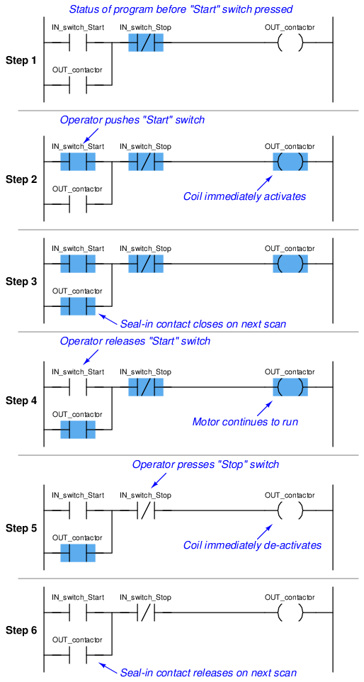
This sequence helps illustrate the order of evaluation or scan order of a Ladder Diagram program. The PLC reads a Ladder Diagram from left to right, top to bottom, in the same general order as a human being reads sentences and paragraphs written in English. However, according to the IEC 61131-3 standard, a PLC program must evaluate (read) all inputs (contacts) to a function before determining the status of a function’s output (coil or coils). In other words, the PLC does not make any decision on how to set the state of a coil until all contacts providing power to that coil have been read. Once a coil’s status has been written to memory, any contacts bearing the same tag name will update with that status on subsequent rungs in the program.
Step 5 in the previous sequence is particularly illustrative. When the human operator presses the “Stop” pushbutton, the input channel for IN_switch_Stop becomes activated, which “opens” the normally-closed virtual contact IN_switch_Stop. Upon the next scan of this program rung, the PLC evaluates all input contacts (IN_switch_Start, IN_switch_Stop, and OUT_contactor) to check their status before deciding what status to write to the OUT_contactor coil. Seeing that the IN_switch_Stop contact has been forced open by the activation of its respective discrete input channel, the PLC writes a “0” (or “False”) state to the OUT_contactor coil. However, the OUT_contactor feedback contact does not update until the next scan, which is why you still see it color-highlighted during step 5.
A potential problem with this system as it is designed is that the human operator loses control of the motor in the event of an “open” wiring failure in either pushbutton switch circuit. For instance, if a wire fell off a screw contact for the “Start” pushbutton switch circuit, the motor could not be started if it was already stopped. Similarly, if a wire fell off a screw contact for the “Stop” pushbutton switch circuit, the motor could not be stopped if it was already running. In either case, a broken wire connection acts the same as the pushbutton switch’s “normal” status, which is to keep the motor in its present state. In some applications, this failure mode would not be a severe problem. In many applications, though, it is quite dangerous to have a running motor that cannot be stopped. For this reason, it is customary to design motor start/stop systems a bit differently from what has been shown here.
In order to build a “fail-stop” motor control system with our PLC, we must first re-wire the pushbutton switch to use its normally-closed (NC) contact:
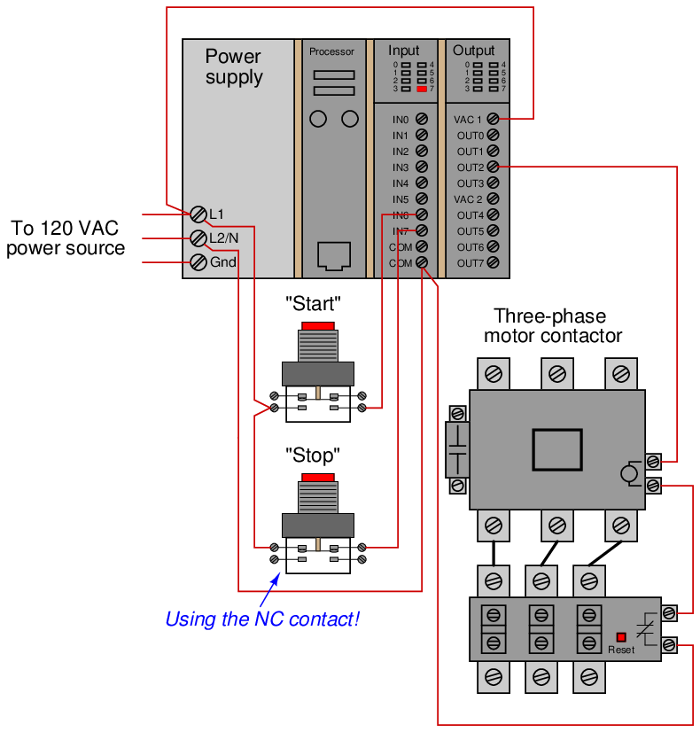
This keeps discrete input channel 7 activated when the pushbutton is unpressed. When the operator presses the “Stop” pushbutton, the switch’s contact will be forced open, and input channel 7 will de-energize. If a wire happens to fall off a screw terminal in the “Stop” switch circuit, input channel 7 will de-energize just the same as if someone pressed the “Stop” pushbutton, which will automatically shut off the motor.
In order for the PLC program to work properly with this new switch wiring, the virtual contact for IN_switch_Stop must be changed from a normally-closed (NC) to a normally-open (NO):
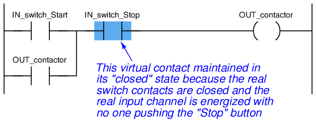
As before, the IN_switch_Stop virtual contact is in the “closed” state when no one presses the “Stop” switch, enabling the motor to start any time the “Start” switch is pressed. Similarly, the IN_switch_Stop virtual contact will open any time someone presses the “Stop” switch, thus stopping virtual “power” from flowing to the OUT_contactor coil.
Although this is a very common way to build PLC-controlled motor start/stop systems – with an NC pushbutton switch and an NO “Stop” virtual contact – students new to PLC programming often find this logical reversal confusing22 . Perhaps the most common reason for this confusion is a mis-understanding of the “normal” concept for switch contacts, be they real or virtual. The IN_switch_Stop virtual contact is programmed to be normally-open (NO), but yet it is typically found in the closed state. Recall that the “normal” status of any switch is its status while in a resting condition of no stimulation, not necessarily its status while the process is in a “normal” operating mode. The “normally-open” virtual contact IN_switch_Stop is typically found in the closed state because its corresponding input channel is typically found energized, owing to the normally-closed pushbutton switch contact, which passes real electrical power to the input channel while no one presses the switch. Just because a switch is configured as normally-open does not necessarily mean it will be typically found in the open state! The status of any switch contact, whether real or virtual, is a function of its configuration (NO versus NC) and the stimulus applied to it.
Another concern surrounding real-world wiring problems is what this system will do if the motor contactor coil circuit opens for any reason. An open circuit may develop as a result of a wire falling off a screw terminal, or it may occur because the thermal overload contact tripped open due to an over-temperature event. The problem with our motor start/stop system as designed is that it is not “aware” of the contactor’s real status. In other words, the PLC “thinks” the contactor will be energized any time discrete output channel 2 is energized, but that may not actually be the case if there is an open fault in the contactor’s coil circuit.
This may lead to a dangerous condition if the open fault in the contactor’s coil circuit is later cleared. Imagine an operator pressing the “Start” switch but noticing the motor does not actually start. Wondering why this may be, he or she goes to look at the overload relay to see if it is tripped. If it is tripped, and the operator presses the “Reset” button on the overload assembly, the motor will immediately start because the PLC’s discrete output has remained energized all the time following the pressing of the “Start” switch. Having the motor start up as soon as the thermal overload is reset may come as a surprise to operations personnel, and this could be quite dangerous if anyone happens to be near the motor-powered machinery when it starts.
What would be safer is a motor control system that refuses to “latch” on unless the contactor actually energizes when the “Start” switch is pressed. For this to be possible, the PLC must have some way of sensing the contactor’s status.
In order to make the PLC “aware” of the contactor’s real status, we may connect the auxiliary switch contact to one of the unused discrete input channels on the PLC, like this:
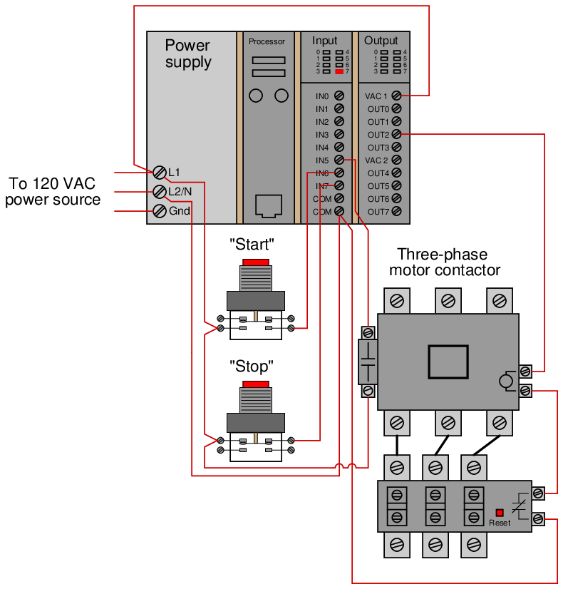
Now, the PLC is able to sense the real-time status of the contactor via input channel 5.
We may modify the PLC program to recognize this status by assigning a new tag name to this input (IN_contactor_aux) and using a normally-open virtual contact of this name as the seal-in contact instead of the OUT_contactor bit:
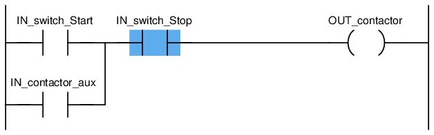
Now, if the contactor fails to energize for any reason when the operator presses the “Start” switch, the PLC’s output will fail to latch when the “Start” switch is released. When the open fault in the contactor’s coil circuit is cleared, the motor will not immediately start up, but rather wait until the operator presses the “Start” switch again, which is a much safer operating characteristic than before.
A special class of virtual “coil” used in PLC ladder programming that bears mentioning is the “latching” coil. These usually come in two forms: a set coil and a reset coil. Unlike a regular “output” coil that positively writes to a bit in the PLC’s memory with every scan of the program, “set” and “reset” coils only write to a bit in memory when energized by virtual power. Otherwise, the bit is allowed to retain its last value.
A very simple motor start/stop program could be written with just two input contacts and two of these latching coils (both bearing the same tag name, writing to the same bit in memory):
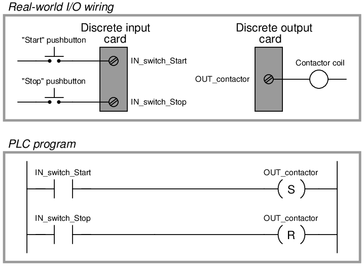
Note the use of a normally-open (NO) pushbutton switch contact (again!), with no auxiliary contact providing status indication of the contactor to the PLC. This is a very minimal program, shown for the strict purpose of illustrating the use of “set” and “reset” latching coils in Ladder Diagram PLC programming.
“Set” and “Reset” coils23 are examples of what is known in the world of PLC programming as retentive instructions. A “retentive” instruction retains its value after being virtually “de-energized” in the Ladder Diagram “circuit.” A standard output coil is non-retentive, which means it does not “latch” when de-energized. The concept of retentive and non-retentive instructions will appear again as we explore PLC programming, especially in the area of timers.
Ordinarily, we try to avoid multiple coils bearing the same label in a PLC Ladder Diagram program. With each coil representing a “write” instruction, multiple coils bearing the same name represents multiple “write” operations to the same bit in the PLC’s memory. Here, with latching coils, there is no conflict because each of the coils only writes to the OUT_contactor bit when its respective contact is energized. So long as only one of the pushbutton switches is actuated at a time, there is no conflict between the identically-named coils.
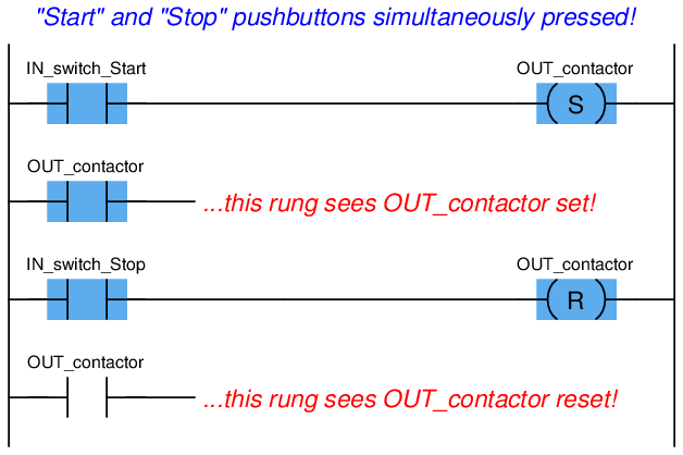
This raises the question: what would happen if both pushbutton switches were simultaneously pressed? What would happen if both “Set” and “Reset” coils were “energized” at the same time? The result is that the OUT_contactor bit would first be “set” (written to a value of 1) then “reset” (written to a value of 0) in that order as the two rungs of the program were scanned from top to bottom. PLCs typically do not typically update their discrete I/O registers while scanning the Ladder Diagram program (this operation takes place either before or after each program scan), so the real discrete output channel status will be whatever the last write operation told it to be, in this case “reset” (0, or off).
Even if the discrete output is not “confused” due to the conflicting write operations of the “Set” and “Reset” coils, other rungs of the program written between the “Set” and “Reset” rungs might be. Consider for example a case where there were other program rungs following the “Set” and “Reset” rungs reading the status of the OUT_contactor bit for some purpose. Those other rungs would indeed become “confused” because they would see the OUT_contactor bit in the “set” state while the actual discrete output of the PLC (and any rungs following the “Reset” rung) would see the OUT_contactor bit in the “reset” state:
Multiple (non-retentive) output coils with the same memory address are almost always a programming faux pax for this reason, but even retentive coils which are designed to be used in matched pairs can cause trouble if the implications of simultaneous energization are not anticipated. Multiple contacts with identical addresses are no problem whatsoever, because multiple “read” operations to the same bit in memory will never cause a conflict.
The IEC 61131-3 PLC programming standard specifies transition-sensing contacts as well as the more customary “static” contacts. A transition-sensing contact will “actuate” only for a duration of one program scan, even if its corresponding bit remains active. Two types of transition-sensing Ladder Diagram contacts are defined in the IEC standard: one for positive transitions and another for negative transitions. The following example shows a wiring diagram, Ladder Diagram program, and a timing diagram demonstrating how each type of transition-sensing contact functions when stimulated by a real (electrical) input signal to a discrete channel:
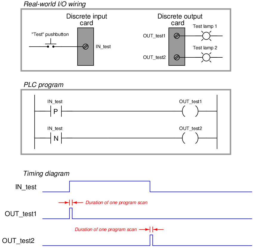
When the pushbutton switch is pressed and the discrete input energized, the first test lamp will blink “on” for exactly one scan of the PLC’s program, then return to its off state. The positive-transition contact (with the letter “P” inside) activates the coil OUT_test1 only during the scan it sees the status of IN_test transition from “false” to “true,” even though the input remains energized for many scans after that transition. Conversely, when the pushbutton switch is released and the discrete input de-energizes, the second test lamp will blink “on” for exactly one scan of the PLC’s program then return to its off state. The negative-transition contact (with the letter “N” inside) activates the coil OUT_test2 only during the scan it sees the status of IN_test transition from “true” to “false,” even though the input remains de-energized for many scans after that transition:
It should be noted that the duration of a single PLC program scan is typically very short: measured in milliseconds. If this program were actually tested in a real PLC, you would probably not be able to see either test lamp light up, since each pulse is so short-lived. Transitional contacts are typically used any time it is desired to execute an instruction just one time following a “triggering” event, as opposed to executing that instruction over and over again so long as the event status is maintained “true.”
Contacts and coils represent only the most basic of instructions in the Ladder Diagram PLC programming language. Many other instructions exist, which will be discussed in the following subsections.
12.4.2 Counters
A counter is a PLC instruction that either increments (counts up) or decrements (counts down) an integer number value when prompted by the transition of a bit from 0 to 1 (“false” to “true”). Counter instructions come in three basic types: up counters, down counters, and up/down counters. Both “up” and “down” counter instructions have single inputs for triggering counts, whereas “up/down” counters have two trigger inputs: one to make the counter increment and one to make the counter decrement.
To illustrate the use of a counter instruction, we will analyze a PLC-based system designed to count objects as they pass down a conveyor belt:
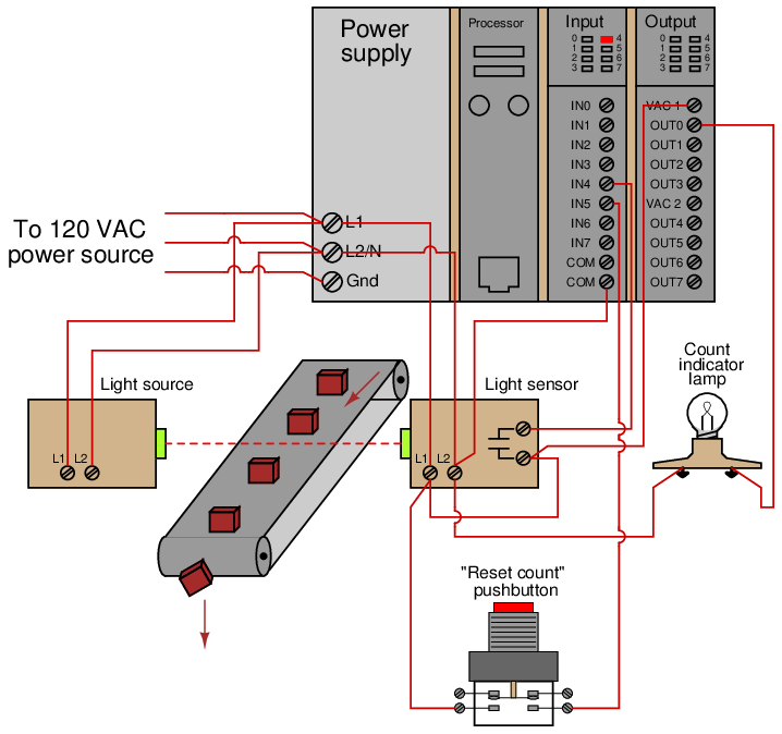
In this system, a continuous (unbroken) light beam causes the light sensor to close its output contact, energizing discrete channel IN4. When an object on the conveyor belt interrupts the light beam from source to sensor, the sensor’s contact opens, interrupting power to input IN4. A pushbutton switch connected to activate discrete input IN5 when pressed will serve as a manual “reset” of the count value. An indicator lamp connected to one of the discrete output channels will serve as an indicator of when the object count value has exceeded some pre-set limit.
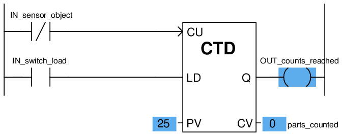
We will now analyze a simple Ladder Diagram program designed to increment a counter instruction each time the light beam breaks:
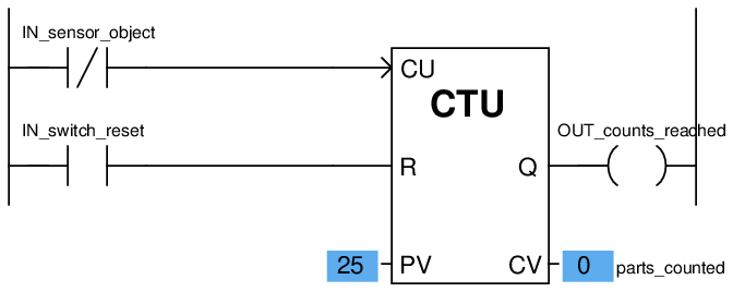
This particular counter instruction (CTU) is an incrementing counter, which means it counts “up” with each off-to-on transition input to its “CU” input. The normally-closed virtual contact (IN_sensor_object) is typically held in the “open” state when the light beam is continuous, by virtue of the fact the sensor holds that discrete input channel energized while the beam is continuous. When the beam is broken by a passing object on the conveyor belt, the input channel de-energizes, causing the virtual contact IN_sensor_object to “close” and send virtual power to the “CU” input of the counter instruction. This increments the counter just as the leading edge of the object breaks the beam. The second input of the counter instruction box (“R”) is the reset input, receiving virtual power from the contact IN_switch_reset whenever the reset pushbutton is pressed. If this input is activated, the counter immediately resets its current value (CV) to zero.
Status indication is shown in this Ladder Diagram program, with the counter’s preset value (PV) of 25 and the counter’s current value (CV) of 0 shown highlighted in blue. The preset value is something programmed into the counter instruction before the system put into service, and it serves as a threshold for activating the counter’s output (Q), which in this case turns on the count indicator lamp (the OUT_counts_reached coil). According to the IEC 61131-3 programming standard, this counter output should activate whenever the current value is equal to or greater than the preset value (Q is active if CV ≥ PV).
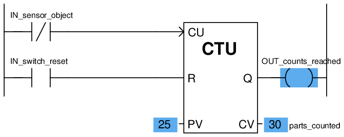
This is the status of the same program after thirty objects have passed by the sensor on the conveyor belt. As you can see, the current value of the counter has increased to 30, exceeding the preset value and activating the discrete output:
If all we did not care about maintaining an accurate total count of objects past 25 – but merely wished the program to indicate when 25 objects had passed by – we could also use a down counter instruction preset to a value of 25, which turns on an output coil when the count reaches zero:
Here, a “load” input causes the counter’s current value to equal the preset value (25) when activated. With each sensor pulse received, the counter instruction decrements. When it reaches zero, the Q output activates.
A potential problem in either version of this object-counting system is that the PLC cannot discriminate between forward and reverse motion on the conveyor belt. If, for instance, the conveyor belt were ever reversed in direction, the sensor would continue to count objects that had already passed by before (in the forward direction) as those objects retreated on the belt. This would be a problem because the system would “think” more objects had passed along the belt (indicating greater production) than actually did.
One solution to this problem is to use an up/down counter, capable of both incrementing (counting up) and decrementing (counting down), and equip this counter with two light-beam sensors capable of determining direction of travel. If two light beams are oriented parallel to each other, closer than the width of the narrowest object passing along the conveyor belt, we will have enough information to determine direction of object travel:
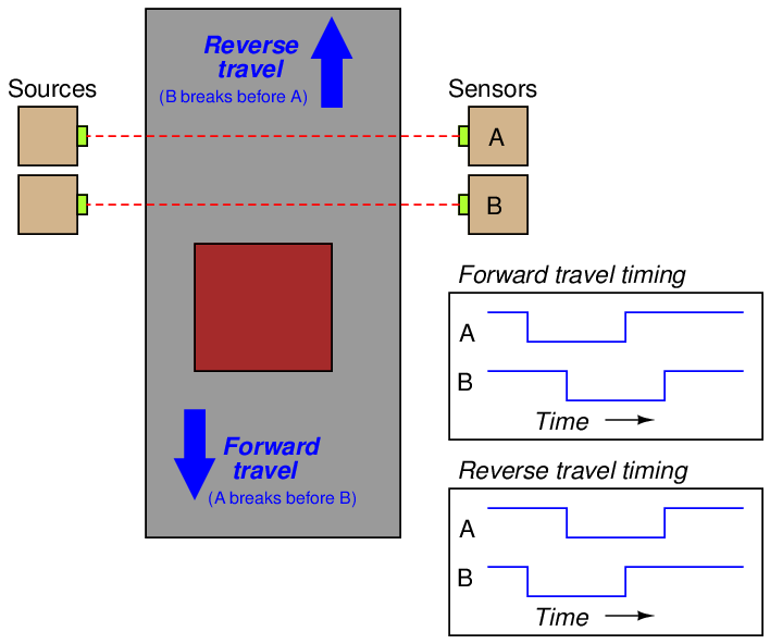
This is called quadrature signal timing, because the two pulse waveforms are approximately 90o (one-quarter of a period) apart in phase. We can use these two phase-shifted signals to increment or decrement an up/down counter instruction, depending on which pulse leads and which pulse lags.
A Ladder Diagram PLC program designed to interpret the quadrature pulse signals is shown here, making use of negative-transition contacts as well as standard contacts:
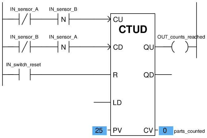
The counter will increment (count up) when sensor B de-energizes only if sensor A is already in the de-energized state (i.e. light beam A breaks before B). The counter will decrement (count down) when sensor A de-energizes only if sensor B is already in the de-energized state (i.e. light beam B breaks before A).
Note that the up/down counter has both a “reset” (R) input and a “load” input (“LD”) to force the current value. Activating the reset input forces the counter’s current value (CV) to zero, just as we saw with the “up” counter instruction. Activating the load input forces the counter’s current value to the preset value (PV), just as we saw with the “down” counter instruction. In the case of an up/down counter, there are two Q outputs: a QU (output up) to indicate when the current value is equal to or greater than the preset value, and a QD (output down) to indicate when the current value is equal to or less than zero.
Note how the current value (CV) of each counter shown is associated with a tag name of its own, in this case parts_counted. The integer number of a counter’s current value (CV) is a variable in the PLC’s memory just like boolean values such as IN_sensor_A and IN_switch_reset, and may be associated with a tag name or symbolic address just the same24 . This allows other instructions in a PLC program to read (and sometimes write!) values from and to that memory location.
12.4.3 Timers
A timer is a PLC instruction measuring the amount of time elapsed following an event. Timer instructions come in two basic types: on-delay timers and off-delay timers. Both “on-delay” and “off-delay” timer instructions have single inputs triggering the timed function.
An “on-delay” timer activates an output only when the input has been active for a minimum amount of time. Take for instance this PLC program, designed to sound an audio alarm siren prior to starting a conveyor belt. To start the conveyor belt motor, the operator must press and hold the “Start” pushbutton for 10 seconds, during which time the siren sounds, warning people to clear away from the conveyor belt that is about to start. Only after this 10-second start delay does the motor actually start (and latch “on”):
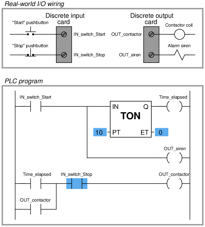
Similar to an “up” counter, the on-delay timer’s elapsed time (ET) value increments once per second until the preset time (PT) is reached, at which time its output (Q) activates. In this program, the preset time value is 10 seconds, which means the Q output will not activate until the “Start” switch has been depressed for 10 seconds. The alarm siren output, which is not activated by the timer, energizes immediately when the “Start” pushbutton is pressed.
An important detail regarding this particular timer’s operation is that it be non-retentive. This means the timer instruction should not retain its elapsed time value when the input is de-activated. Instead, the elapsed time value should reset back to zero every time the input de-activates. This ensures the timer resets itself when the operator releases the “Start” pushbutton. A retentive on-delay timer, by contrast, maintains its elapsed time value even when the input is de-activated. This makes it useful for keeping “running total” times for some event.
Most PLCs provide retentive and non-retentive versions of on-delay timer instructions, such that the programmer may choose the proper form of on-delay timer for any particular application. The IEC 61131-3 programming standard, however, addresses the issue of retentive versus non-retentive timers a bit differently. According to the IEC 61131-3 standard, a timer instruction may be specified with an additional enable input (EN) that causes the timer instruction to behave non-retentively when activated, and retentively when de-activated. The general concept of the enable (EN) input is that the instruction behaves “normally” so long as the enable input is active (in this case, non-retentive timing action is considered “normal” according to the IEC 61131-3 standard), but the instruction “freezes” all execution whenever the enable input de-activates. This “freezing” of operation has the effect of retaining the current time (CT) value even if the input signal de-activates.
For example, if we wished to add a retentive timer to our conveyor control system to record total run time for the conveyor motor, we could do so using an “enabled” IEC 61131-3 timer instruction like this:
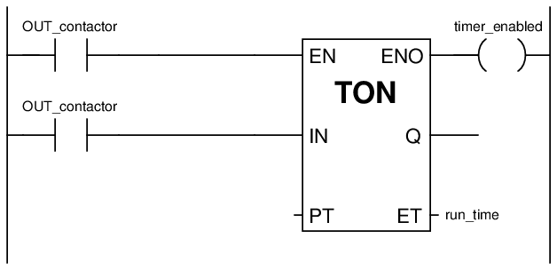
When the motor’s contactor bit (OUT_contactor) is active, the timer is enabled and allowed to time. However, when that bit de-activates (becomes “false”), the timer instruction as a whole is disabled, causing it to “freeze” and retain its current time (CT) value25 . This allows the motor to be started and stopped, with the timer maintaining a tally of total motor run time.
If we wished to give the operator the ability to manually reset the total run time value to zero, we could hard-wire an additional switch to the PLC’s discrete input card and add “reset” contacts to the program like this:
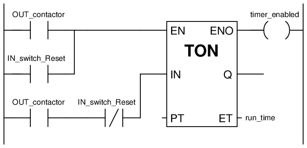
Whenever the “Reset” switch is pressed, the timer is enabled (EN) but the timing input (IN) is disabled, forcing the timer to (non-retentively) reset its current time (CT) value to zero.
The other major type of PLC timer instruction is the off-delay timer. This timer instruction differs from the on-delay type in that the timing function begins as soon as the instruction is de-activated, not when it is activated. An application for an off-delay timer is a cooling fan motor control for a large industrial engine. In this system, the PLC starts an electric cooling fan as soon as the engine is detected as rotating, and keeps that fan running for two minutes following the engine’s shut-down to dissipate residual heat:
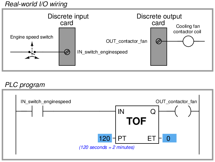
When the input (IN) to this timer instruction is activated, the output (Q) immediately activates (with no time delay at all) to turn on the cooling fan motor contactor. This provides the engine with cooling as soon as it begins to rotate (as detected by the speed switch connected to the PLC’s discrete input). When the engine stops rotating, the speed switch returns to its normally-open position, de-activating the timer’s input signal which starts the timing sequence. The Q output remains active while the timer counts from 0 seconds to 120 seconds. As soon as it reaches 120 seconds, the output de-activates (shutting off the cooling fan motor) and the elapsed time value remains at 120 seconds until the input re-activates, at which time it resets back to zero.
The following timing diagrams compare and contrast on-delay with off-delay timers:
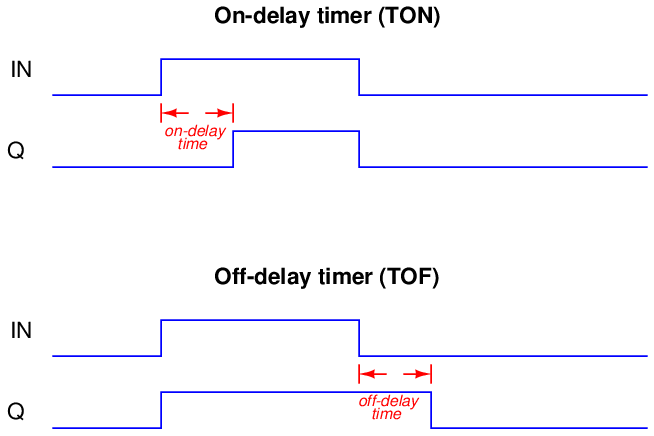
While it is common to find on-delay PLC instructions offered in both retentive and non-retentive forms within the instruction sets of nearly every PLC manufacturer and model, it is almost unheard of to find retentive off-delay timer instructions. Typically, off-delay timers are non-retentive only26 .
12.4.4 Data comparison instructions
As we have seen with counter and timers, some PLC instructions generate digital values other than simple Boolean (on/off) signals. Counters have current value (CV) registers and timers have elapsed time (ET) registers, both of which are typically integer number values. Many other PLC instructions are designed to receive and manipulate non-Boolean values such as these to perform useful control functions.
The IEC 61131-3 standard specifies a variety of data comparison instructions for comparing two non-Boolean values, and generating Boolean outputs. The basic comparative operations of “less than” (<), “greater than” (>), “less than or equal to” (≤), “greater than or equal to” (≥), “equal to” (=), and “not equal to” (≠) may be found as a series of “box” instructions in the IEC standard:
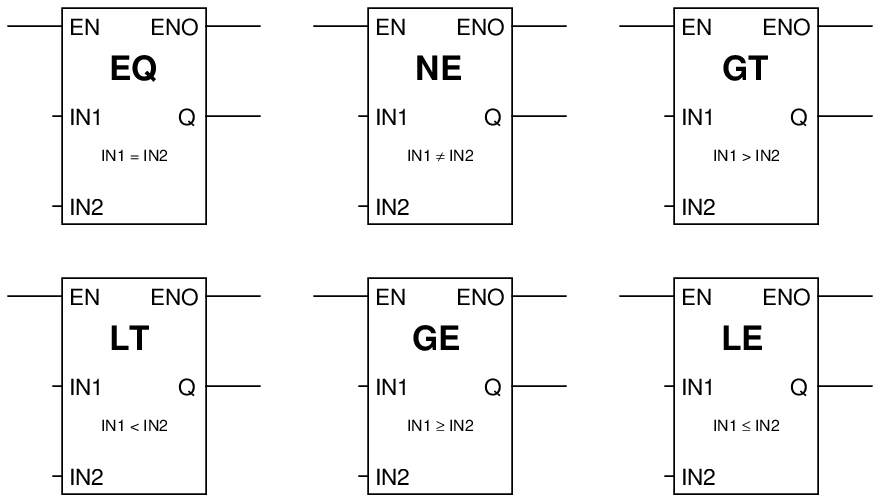
The Q output for each instruction “box” activates whenever the evaluated comparison function is “true” and the enable input (EN) is active. If the enable input remains active but the comparison function is false, the Q output de-activates. If the enable input de-de-activates, the Q output retains its last state.
A practical application for a comparative function is something called alternating motor control, where the run-times of two redundant electric motors27 are monitored, with the PLC determining which motor to turn on next based on which motor has run the least:
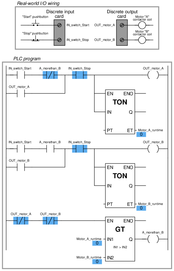
In this program, two retentive on-delay timers keep track of each electric motor’s total run time, storing the run time values in two registers in the PLC’s memory: Motor_A_runtime and Motor_B_runtime. These two integer values are input to the “greater than” instruction box for comparison. If motor A has run longer than motor B, motor B will be the one enabled to start up next time the “start” switch is pressed. If motor A has run less time or the same amount of time as motor B (the scenario shown by the blue-highlighted status indications), motor A will be the one enabled to start. The two series-connected virtual contacts OUT_motor_A and OUT_motor_B ensure the comparison between motor run times is not made until both motors are stopped. If the comparison were continually made, a situation might arise where both motors would start if someone happened to press the Start pushbutton with one motor is already running.
12.4.5 Math instructions
The IEC 61131-3 standard specifies several dedicated ladder instructions for performing arithmetic calculations. Some of them are shown here:
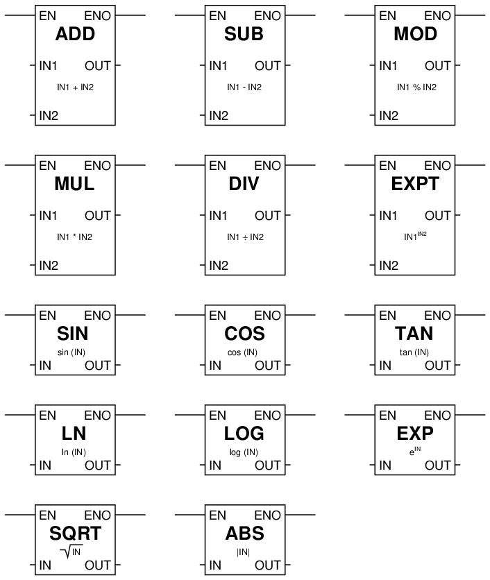
As with the data comparison instructions, each of these math instructions must be enabled by an “energized” signal to the enable (EN) input. Input and output values are linked to each math instruction by tag name.
An example showing the use of such instructions is shown here, converting a temperature measurement in units of degrees Fahrenheit to units of degrees Celsius. In this particular case, the program inputs a temperature measurement of 138 oF and calculates the equivalent temperature of 58.89 oC:
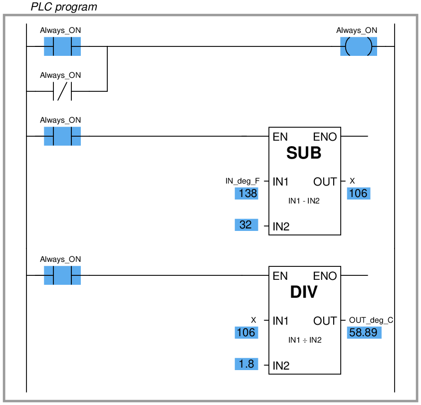
Note how two separate math instructions were required to perform this simple calculation, as well as a dedicated variable (X) used to store the intermediate calculation between the subtraction and the division “boxes.”
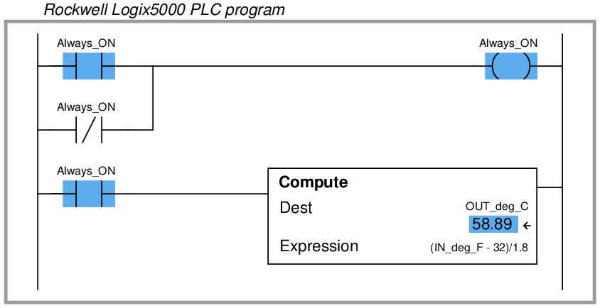
Although not specified in the IEC 61131-3 standard, many programmable logic controllers support Ladder Diagram math instructions allowing the direct entry of arbitrary equations. Rockwell (Allen-Bradley) Logix5000 programming, for example, has the “Compute” (CPT) function, which allows any typed expression to be computed in a single instruction as opposed to using several dedicated math instructions such as “Add,” “Subtract,” etc. General-purpose math instructions dramatically shorten the length of a ladder program compared to the use of dedicated math instructions for any applications requiring non-trivial calculations.
For example, the same Fahrenheit-to-Celsius temperature conversion program implemented in Logix5000 programming only requires a single math instruction and no declarations of intermediate variables:
12.4.6 Sequencers
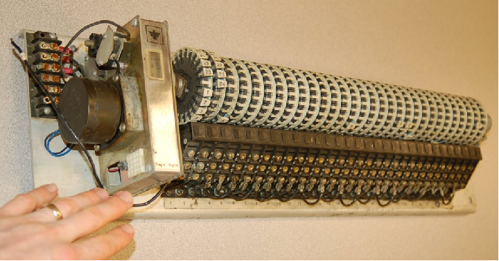
Many industrial processes require control actions to take place in certain, predefined sequences. Batch processes are perhaps the most striking example of this, where materials for making a batch must be loaded into the process vessels, parameters such as temperature and pressure controlled during the batch processing, and then discharge of the product monitored and controlled. Before the advent of reliable programmable logic devices, this form of sequenced control was usually managed by an electromechanical device known as a drum sequencer. This device worked on the principle of a rotating cylinder (drum) equipped with tabs to actuate switches as the drum rotated into certain positions. If the drum rotated at a constant speed (turned by a clock motor), those switches would actuate according to a timed schedule28 .
The following photograph shows a drum sequencer with 30 switches. Numbered tabs on the circumference of the drum mark the drum’s rotary position in one of 24 increments. With this number of switches and tabs, the drum can control up to thirty discrete (on/off) devices over a series of twenty-four sequenced steps:
A typical application for a sequencer is to control a Clean In Place (CIP) system for a food processing vessel, where a process vessel must undergo a cleaning cycle to purge it of any biological matter between food processing cycles. The steps required to clean the vessel are well-defined and must always occur in the same sequence in order to ensure hygienic conditions. An example timing chart is shown here:
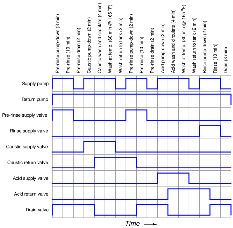
In this example, there are nine discrete outputs – one for each of the nine final control elements (pumps and valves) – and seventeen steps to the sequence, each one of them timed. In this particular sequence, the only input is the discrete signal to commence the CIP cycle. From the initiation of the CIP to its conclusion two and a half hours (150 minutes) later, the sequencer simply steps through the programmed routine.
Another practical application for a sequencer is to implement a Burner Management System (BMS), also called a flame safety system. Here, the sequencer manages the safe start-up of a combustion burner: beginning by “purging” the combustion chamber with fresh air to sweep out any residual fuel vapors, waiting for the command to light the fire, energizing a spark ignition system on command, and then continuously monitoring for presence of good flame and proper fuel supply pressure once the burner is lit.
In a general sense, the operation of a drum sequencer is that of a state machine: the output of the system depends on the condition of the machine’s internal state (the drum position), not just the conditions of the input signals. Digital computers are very adept at implementing state functions, and so the general function of a drum sequencer should be (and is) easy to implement in a PLC. Other PLC functions we have seen (“latches” and timers in particular) are similar, in tha12.4 Ladder Diagram (LD) programmingt the PLC’s output at any given time is a function of both its present input condition(s) and its past input condition(s). Sequencing functions expand upon this concept to define a much larger number of possible states (“positions” of a “drum”), some of which may even be timed.
Unfortunately, despite the utility of drum sequence functions and their ease of implementation in digital form, there seems to be very little standardization between PLC manufacturers regarding sequencing instructions. Sadly, the IEC 61131-3 standard (at least at the time of this writing, in 2009) does not specifically define a sequencing function suitable for Ladder Diagram programming. PLC manufacturers are left to invent sequencing instructions of their own design. What follows here is an exploration of some different sequencer instructions offered by PLC manufacturers.
Koyo “drum” instructions
The drum instruction offered in Koyo PLCs is a model of simplicity itself. This instruction is practically self-explanatory, as shown in the following example:
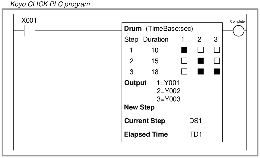
The three-by-three grid of squares represent steps in the sequence and bit states for each step. Rows represent steps, while columns represent output bits written by the drum instruction. In this particular example, a three-step sequence proceeds at the command of a single input (X001), and the drum instruction’s advance from one step to the next proceeds strictly on the basis of elapsed time (a time base orientation). When the input is active, the drum proceeds through its timed sequence. When the input is inactive, the drum halts wherever it left off, and resumes timing as soon as the input becomes active again.
Being based on time, each step in the drum instruction has a set time duration for completion. The first step in this particular example has a duration of 10 seconds, the second step 15 seconds, and the third step 18 seconds. At the first step, only output bit Y001 is set. In the second step, only output bit Y002 is set. In the third step, output bits Y002 and Y003 are set (1), while bit Y001 is reset (0). The colored versus uncolored boxes reveal which output bits are set and reset with each step. The current step number is held in memory register DS1, while the elapsed time (in seconds) is stored in timer register TD1. A “complete” bit is set at the conclusion of the three-step sequence.
Koyo drum instructions may be expanded to include more than three steps and more than three output bits, with each of those step times independently adjustable and each of the output bits arbitrarily assigned to any writable bit addresses in the PLC’s memory.
This next example of a Koyo drum instruction shows how it may be set up to trigger on events rather than on elapsed times. This orientation is called an event base:
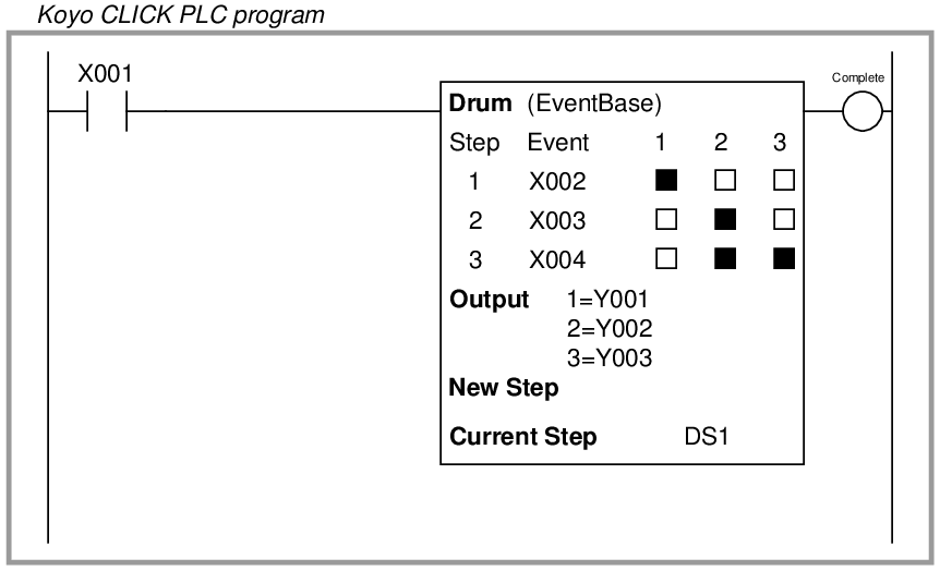
Here, a three-step sequence proceeds when enabled by a single input (X001), with the drum instruction’s advance from one step to the next proceeding only as the different event condition bits become set. When the input is active, the drum proceeds through its sequence when each event condition is met. When the input is inactive, the drum halts wherever it left off regardless of the event bit states.
For example, during the first step (when only output bit Y001 is set), the drum instruction waits for the first condition input bit X002 to become set (1) before proceeding to step 2, with time being irrelevant. When this happens, the drum immediately advances to step 2 and waits for input bit X003 to be set, and so forth. If all three event conditions were met simultaneously (X002, X003, and X004 all set to 1), the drum would skip through all steps as fast as it could (one step per PLC program scan) with no appreciable time elapsed for each step. Conversely, the drum instruction will wait as long as it must for the right condition to be met before advancing, whether that event takes place in milliseconds or in days.
Allen-Bradley sequencer instructions
Rockwell (Allen-Bradley) PLCs use a more sophisticated set of instructions to implement sequences. The closest equivalent to Koyo’s drum instruction is the Allen-Bradley SQO (Sequencer Output) instruction, shown here:
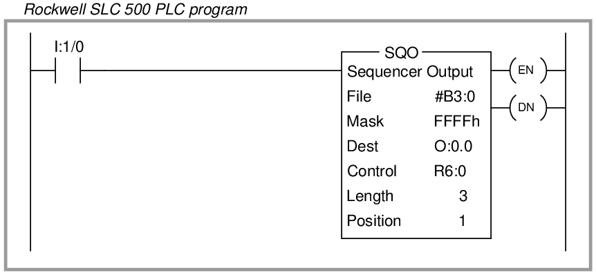
You will notice there are no colored squares inside the SQO instruction box to specify when certain bits are set or reset throughout the sequence, in contrast to the simplicity of the Koyo PLC’s drum instruction. Instead, the Allen-Bradley SQO instruction is told to read a set of 16-bit words beginning at a location in the PLC’s memory arbitrarily specified by the programmer, one word at a time. It steps to the next word in that set of words with each new position (step) value. This means Allen-Bradley sequencer instructions rely on the programmer already having pre-loaded an area of the PLC’s memory with the necessary 1’s and 0’s defining the sequence. This makes the Allen-Bradley sequencer instruction more challenging for a human programmer to interpret because the bit states are not explicitly shown inside the SQO instruction box, but it also makes the sequencer far more flexible in that these bits are not fixed parameters of the SQO instruction and therefore may be dynamically altered as the PLC runs. With the Koyo drum instruction, the assigned output states are part of the instruction itself, and are therefore fixed once the program is downloaded to the PLC (i.e. they cannot be altered without editing and re-loading the PLC’s program). With the Allen-Bradley, the on-or-off bit states for the sequence may be freely altered29 during run-time. This is a very useful feature in recipe-control applications, where the recipe is subject to change at the whim of production personnel, and they would rather not have to rely on a technician or an engineer to re-program the PLC for each new recipe.
The “Length” parameter tells the SQO instruction how many words will be read (i.e. how many steps are in the entire sequence). The sequencer advances to each new position when its enabling input transitions from inactive to active (from “false” to “true”), just like a count-up (CTU) instruction increments its accumulator value with each new false-to-true transition of the input. Here we see another important difference between the Allen-Bradley SQO instruction and the Koyo drum instruction: the Allen-Bradley instruction is fundamentally event-driven, and does not proceed on its own like the Koyo drum instruction is able to when configured for a time base.
Sequencer instructions in Allen-Bradley PLCs use a notation called indexed addressing to specify the locations in memory for the set of 16-bit words it will read. In the example shown above, we see the “File” parameter specified as #B3:0. The “#” symbol tells the instruction that this is a starting location in memory for the first 16-bit word, when the instruction’s position value is zero. As the position value increments, the SQO instruction reads 16-bit words from successive addresses in the PLC’s memory. If B3:0 is the word referenced at position 0, then B3:1 will be the memory address read at position 1, B3:2 will be the memory address read at position 2, etc. Thus, the “position” value causes the SQO instruction to “point” or “index” to successive memory locations.
The bits read from each indexed word in the sequence are compared against a static mask30 specifying which bits in the indexed word are relevant. At each position, only these bits are written to the destination address.
As with most other Allen-Bradley instructions, the sequencer requires the human programmer to declare a special area in memory reserved for the instruction’s internal use. The “R6” file exists just for this purpose, each element in that file holding bit and integer values associated with a sequencer instruction (e.g. the “enable” and “done” bits, the array length, the current position, etc.).
To illustrate, let us examine a set of bits held in the B3 file of an Allen-Bradley SLC 500 PLC, showing how each row (element) of this data file would be read by an SQO instruction as it stepped through its positions:
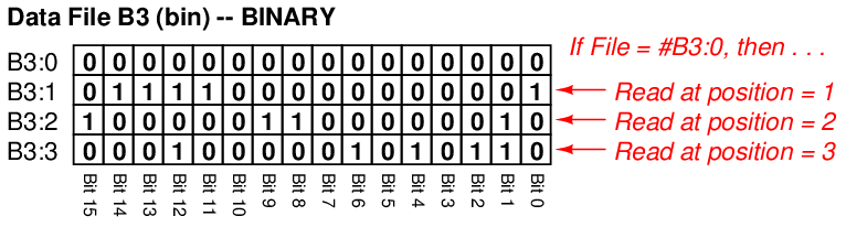
The sequencer’s position number is added to the file reference address as an offset. Thus, if the data file is specified in the SQO instruction box as #B3:0, then B3:1 will be the row of bits read when the sequencer’s position value is 1, B3:2 will be the row of bits read when the position value is 2, and so on.
The mask value specified in the SQO instruction tells the instruction which bits out of each row will be copied to the destination address. A mask value of FFFFh (FFFF in hexadecimal format) means all 16 bits of each B3 word will be read and written to the destination. A mask value of 0001h means only the first (least-significant) bit will be read and written, with the rest being ignored.
Let’s see what would happen with an SQO instruction having a mask value of 000Fh, starting from file index #B3:0, and writing to a destination that is output register O:0.0, given the bit array values in file B3 shown above:
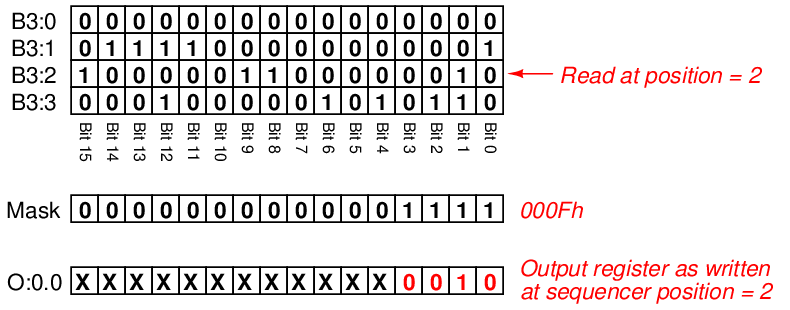
When this SQO instruction is at position 2, it reads the bit values 0010 from B3:2 and writes only those four bits to O:0.0. The “X” symbols shown in the illustration mean that all the other bits in that output register are untouched – the SQO instruction does not write to those bits because they are “masked off” from being written. You may think of the mask’s zero bits inhibiting source bits from being written to the destination word in the same sense that masking tape prevents paint from being applied to a surface.
The following Allen-Bradley SLC 500 PLC program shows how a pair of SQO instructions plus an on-delay timer instruction may be used to duplicate the exact same functionality as the “time base” Koyo drum instruction presented earlier:
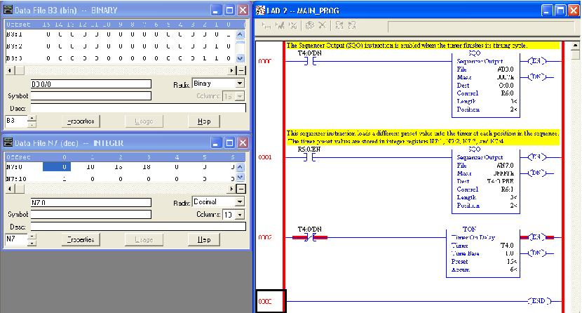
The first SQO instruction reads bits12.4 Ladder Diagram (LD) programming in the B3 file array, sending only the three least-significant of them to the output register O:0.0 (as specified by the 0007h mask value). The second SQO instruction reads integer number values from elements of the N7 integer file and places them into the “preset” register of timer T4:0, so as to dynamically update the timer’s preset value with each step of the sequence. The timer, in turn, counts off each of the time delays and then enables both sequencers to advance to the next position when the specified time has elapsed. Here we see a tremendous benefit of the SQO instruction’s indexed memory addressing: the fact that the SQO instruction reads its bits from arbitrarily-specified memory addresses means we may use SQO instructions to sequence any type of data existing in the PLC’s memory! We are not limited to turning on and off individual bits as we are with the Koyo drum instruction, but rather are free to index whole integer numbers, ASCII characters, or any other forms of binary data resident in the PLC’s memory.
Data file windows appear on the computer screen showing the bit array held in the B3 file as well as the timer values held in the N7 file. In this live screenshot, we see both sequencer instructions at position 2, with the second SQO instruction having loaded a value of 15 seconds from register N7:2 to the timer’s preset register T4:0.PRE.
Note how the enabling contact address for the second SQO instruction is the “enable” bit of the first instruction, ensuring both instructions are enabled simultaneously. This keeps the two separate sequencers synchronized (on the same step).
Event-based transitions may be implemented in Allen-Bradley PLCs using a complementary sequencing instruction called SQC (Sequencer Compare). The SQC instruction is set up very similar to the SQO instruction, with an indexed file reference address to read from, a reserved memory structure for internal use, a set length, and a position value. The purpose of the SQC instruction is to read a data register and compare it against another data register, setting a “found” (FD) bit if the two match. Thus, the SQC instruction is ideally suited for detecting when certain conditions have been met, and thus may be used to enable an SQO instruction to proceed to the next step in its sequence.
The following program example shows an Allen-Bradley MicroLogix 1100 PLC programmed with both an SQO and an SQC instruction:
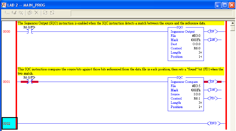
The three-position SQO (Sequencer Output) instruction reads data from B3:1, B3:2, and B3:3, writing the four least-significant of those bits to output register O:0.0. The three-position SQC (Sequencer Compare) instruction reads data from B3:6, B3:7, and B3:8, comparing the four least-significant of those bits against input bits in register I:0.0. When the four input bit conditions match the selected bits in the B3 file, the SQC instruction’s FD bit is set, causing both the SQO instruction and the SQC instruction to advance to the next step.
Lastly, Allen-Bradley PLCs offer a third sequencing instruction called Sequencer Load (SQL), which performs the opposite function as the Sequencer Output (SQO). An SQL instruction takes data from a designated source and writes it into an indexed register according to a position count value, rather than reading data from an indexed register and sending it to a designated destination as does the SQO instruction. SQL instructions are useful for reading data from a live process and storing it in different registers within the PLC’s memory at different times, such as when a PLC is used for datalogging (recording process data).
12.5 Structured Text (ST) programming
(Will be addressed in future versions of this book)
12.6 Instruction List (IL) programming
(Will be addressed in future versions of this book)
12.7 Function Block Diagram (FBD) programming
(Will be addressed in future versions of this book)
12.8 Sequential Function Chart (SFC) programming
(Will be addressed in future versions of this book)