
A fundamental limitation of proportional control has to do with its response to changes in setpoint and changes in process load. A “load” in a controlled process is any variable not controlled by the loop controller which nevertheless affects the process variable the controller is trying to regulate. In other words, a “load” is any factor the loop controller must compensate for while maintaining the process variable at setpoint.
In our hypothetical heat exchanger system, the temperature of the incoming process fluid is an example of a load:
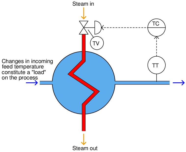
If the incoming fluid temperature were to suddenly decrease, the immediate effect this would have on the process would be to decrease the outlet temperature (which is the temperature we are trying to maintain at a steady value). It should make intuitive sense that a colder incoming fluid will require more heat input to raise it to the same outlet temperature as before. If the heat input remains the same (at least in the immediate future), this colder incoming flow must make the outlet flow colder than it was before. Thus, incoming feed temperature has an impact on the outlet temperature whether we like it or not, and the control system must compensate for these unforeseen and uncontrolled changes. This is precisely the definition of a “load”: a burden3 on the control system.
Of course, it is the job of the controller to counteract any tendency for the outlet temperature to stray from setpoint, but as we shall soon see this cannot be perfectly achieved with proportional control alone.
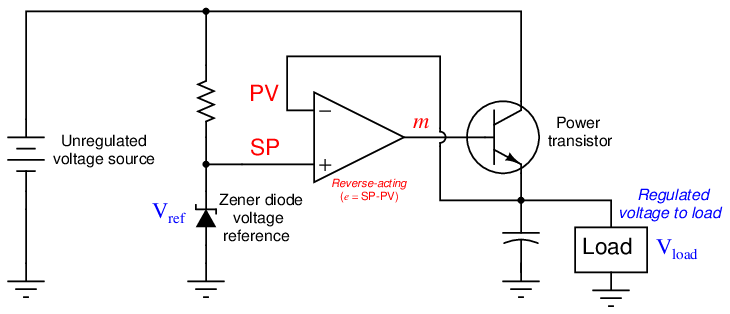
Let us perform a “thought experiment” to demonstrate this phenomenon of proportional-only offset. Imagine the controller has been controlling outlet temperature exactly at setpoint (PV = SP), and then suddenly the inlet feed temperature drops and remains colder than before. Recall that the equation for a reverse-acting proportional controller is as follows:
Where,
m = Controller output
Kp = Proportional gain
SP = Setpoint
PV = Process variable
b = Bias
The introduction of colder feed fluid to the heat exchanger makes the outlet temperature (PV) begin to fall. As the PV falls, the controller calculates a positive error (SP − PV). This positive error, when multiplied by the controller’s gain value, drives the output to a greater value. This opens up the steam valve, adding more heat to the exchanger.
As more heat is added, the rate of temperature drop slows down. The further the PV drops, the more the steam valve opens, until enough additional heat is being added to the heat exchanger to maintain a constant outlet temperature. However, this new stable PV value will be less than it was prior to the introduction of colder feed (i.e. less than the SP). In fact, the controller’s automatic action can never return the PV to its original (SP) value so long as the feed remains colder than before. The reason for this is that a greater flow of steam is necessary to balance a colder feed coming in, and the only way a proportional controller is ever going to automatically drive the steam valve to this greater-flow position is if an error develops between PV and SP. Thus, an offset inevitably develops between PV and SP due to the load (colder feed).
We may prove the inevitability of this offset another way: imagine somehow that the PV did actually return to the SP value despite the colder feed fluid (remaining colder). If this happened, the steam valve would also return to its former throttling position where it was before the feed temperature dropped. However, we know that this former position will not allow enough steam through to the exchanger to overcome the colder feed – if it did, the PV never would have decreased to begin with! A further-open valve is precisely what we need to stabilize the PV given this colder feed, yet the only way the proportional-only controller can achieve this is if the PV actually falls below SP.
To summarize: the only way a proportional-only controller can automatically generate a new output value (m) is if the PV deviates from SP. Therefore, load changes (requiring new output values to compensate) force the PV to deviate from SP.
Another “thought experiment” may be helpful to illustrate the phenomenon of proportional-only offset. Imagine building your own cruise control system for your automobile based on the proportional-only equation: the engine’s throttle position is a function of the difference between PV (road speed) and SP (the desired “target” speed). Let us further suppose that you carefully adjust the bias value of your cruise control system to achieve PV = SP on level ground at a speed of 70 miles per hour (70% on a 0 to 100 MPH speedometer scale), with the throttle at a position of 40%, and a gain (Kp) of 2:


Imagine now that after cruising precisely at setpoint (70% = 70 MPH), the road begins to incline uphill for several miles. This, obviously, is a load on the cruise control system. With the cruise control disengaged, the automobile would slow down because the same throttle position (40%) sufficient to maintain setpoint (70 MPH) on level ground is not enough power to maintain that same setpoint on an incline.
With the cruise control engaged, the engine throttle will automatically open further as speed drops. At a speed of 69 MPH, the throttle opens up to 42%. At a speed of 68 MPH, the throttle opens up to 44%. Every drop in speed of 1 MPH results in a 2% further-open throttle to send more power to the wheels.
Suppose the demands of this particular inclined road require a 50% throttle position for this automobile to maintain a constant speed. In order for your proportional-only cruise control system to deliver this necessary 50% throttle position, the speed will have to “droop” by 5 MPH below setpoint:


There is simply no other way for your proportional-only controller to automatically achieve the requisite 50% throttle position aside from letting the speed sag below setpoint by 5% (5 MPH). Given this fact, the only way the proportional-only cruise control will ever return the speed to setpoint (70 MPH) is if and when the load conditions change to allow for a lesser throttle position of 40%. So long as the load demands a different throttle position than the bias value, the speed must deviate from the setpoint value of 70 MPH.
This necessary error developing between PV and SP is called proportional-only offset, sometimes called droop. The amount of droop depends on how severe the load change is, and how aggressive the controller responds (i.e. how much gain it has). The term “droop” is very misleading, as it is possible for the error to develop the other way (i.e. the PV might rise above SP due to a load change!). Imagine the opposite load-change scenario in our steam heat exchanger process, where the incoming feed temperature suddenly rises instead of falls. If the controller was controlling exactly at setpoint before this upset, the final result will be an outlet temperature that settles at some point above setpoint, enough so the controller is able to pinch the steam valve far enough closed to stop any further rise in temperature.
Proportional-only offset also occurs as a result of setpoint changes. We could easily imagine the same sort of effect following an operator’s increase of setpoint for the temperature controller on the heat exchanger. After increasing the setpoint, the controller immediately increases the output signal, sending more steam to the heat exchanger. As temperature rises, though, the proportional algorithm causes the output signal to decrease. When the rate of heat energy input by the steam equals the rate of heat energy carried away from the heat exchanger by the heated fluid (a condition of energy balance), the temperature stops rising. This new equilibrium temperature will not be at setpoint, assuming the temperature was holding at setpoint prior to the human operator’s setpoint increase. The new equilibrium temperature indeed cannot ever achieve any setpoint value higher than the one it did in the past, for if the error ever returned to zero (PV = SP), the steam valve would return to its old position, which we know would be insufficient to raise the temperature of the heated fluid to a new value.
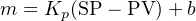
An example of proportional-only control in the context of electronic power supply circuits is the following opamp voltage regulator, used to stabilize voltage to a load with power supplied by an unregulated voltage source:
In this circuit, a zener diode establishes a “reference” voltage (which may be thought of as a “setpoint” for the controlling opamp to follow). The operational amplifier acts as the proportional-only controller, sensing voltage at the load (PV), and sending a driving output voltage to the base of the power transistor to keep load voltage constant despite changes in the supply voltage or changes in load current (both “loads” in the process-control sense of the word, since they tend to influence voltage at the load circuit without being under the control of the opamp).
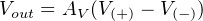
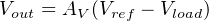
If everything functions properly in this voltage regulator circuit, the load’s voltage will be stable over a wide range of supply voltages and load currents. However, the load voltage cannot ever precisely equal the reference voltage established by the zener diode, even if the operational amplifier (the “controller”) is without defect. The reason for this incapacity to perfectly maintain “setpoint” is the simple fact that in order for the opamp to generate any output signal at all, there absolutely must be a differential voltage between the two input terminals for the amplifier to amplify. Operational amplifiers (ideally) generate an output voltage equal to the enormously high gain value (AV ) multiplied by the difference in input voltages (in this case, V ref − V load). If V load (the “process variable”) were to ever achieve equality with V ref (the “setpoint”), the operational amplifier would experience absolutely no differential input voltage to amplify, and its output signal driving the power transistor would fall to zero. Therefore, there must always exist some offset between V load and V ref (between process variable and setpoint) in order to give the amplifier some input voltage to amplify.
The amount of offset is ridiculously small in such a circuit, owing to the enormous gain of the operational amplifier. If we take the opamp’s transfer function to be V out = AV (V (+) −V (−)), then we may set up an equation predicting the load voltage as a function of reference voltage (assuming a constant 0.7 volt drop between the base and emitter terminals of the transistor):


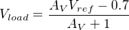
If, for example, our zener diode produced a reference voltage of 5.00000 volts and the operational amplifier had an open-loop voltage gain of 250000, the load voltage would settle at a theoretical value of 4.9999772 volts: just barely below the reference voltage value. If the opamp’s open-loop voltage gain were much less – say only 100 – the load voltage would only be 4.94356 volts. This still is quite close to the reference voltage, but definitely not as close as it would be with a greater opamp gain!
Clearly, then, we can minimize proportional-only offset by increasing the gain of the process controller gain (i.e. decreasing its proportional band). This makes the controller more “aggressive” so it will move the control valve further for any given change in PV or SP. Thus, not as much error needs to develop between PV and SP to move the valve to any new position it needs to go. However, too much controller gain makes the control system unstable: at best it will exhibit residual oscillations after setpoint and load changes, and at worst it will oscillate out of control altogether. Extremely high gains work well to minimize offset in operational amplifier circuits, only because time delays are negligible between output and input. In applications where large physical processes are being controlled (e.g. furnace temperatures, tank levels, gas pressures, etc.) rather than voltages across small electronic loads, such high controller gains would be met with debilitating oscillations.
If we are limited in how much gain we can program in to the controller, how do we minimize this offset? One way is for a human operator to periodically place the controller in manual mode and move the control valve just a little bit more so the PV once again reaches SP, then place the controller back into automatic mode. In essence this technique adjusts the “Bias” term of the controller equation. The disadvantage of this technique is rather obvious: it requires human intervention. What is the point of having an automation system requiring periodic human intervention to maintain setpoint?
A more sophisticated method for eliminating proportional-only offset is to add a different control action to the controller: one that takes action based on the amount of error between PV and SP and the amount of time that error has existed. We call this control mode integral, or reset.