
RTDs are completely passive sensing elements, requiring the application of an externally-sourced electric current in order to function as temperature sensors. Thermocouples, however, generate their own electric potential. In some ways, this makes thermocouple systems simpler because the device receiving the thermocouple’s signal does not have to supply electric power to the thermocouple. It also makes thermocouple systems potentially safer than RTDs in applications where explosive compounds may exist in the atmosphere, because the power levels generated by a thermocouple tend to be less than the power levels dissipated by an RTD. The self-powering nature of thermocouples also means they do not suffer from the same “self-heating” effect as RTDs.
In other ways, however, thermocouple circuits are more complex and troublesome than RTD circuits because the generation of voltage actually occurs in two different locations within the circuit, not simply at the sensing point. This means the receiving circuit must “compensate” for temperature in another location in order to accurately measure temperature in the desired location.
Though typically not as accurate as RTDs, thermocouples are more rugged, have greater temperature measurement spans, and are easier to manufacture in different physical forms.
21.4.1 Dissimilar metal junctions
When two dissimilar metal wires are joined together at one end, a voltage is produced at the other end that is approximately proportional to temperature. That is to say, the junction of two different metals behaves like a temperature-sensitive battery. This form of electrical temperature sensor is called a thermocouple:
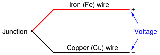
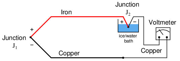
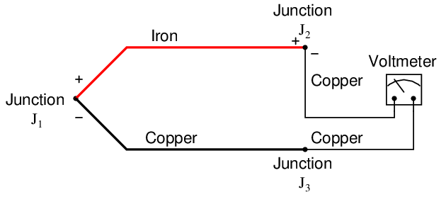
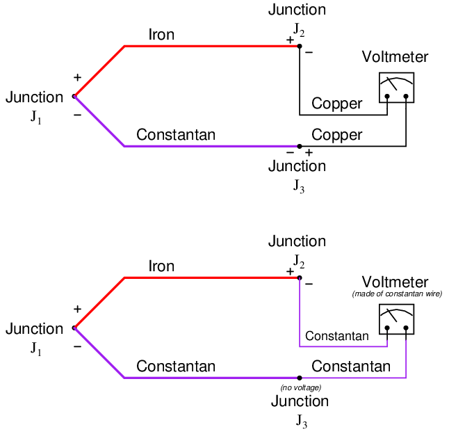
This phenomenon provides us with a simple way to electrically infer temperature: simply measure the voltage produced by the junction, and you can tell the temperature of that junction. And it would be that simple, if it were not for an unavoidable consequence of electric circuits: when we connect any kind of electrical instrument to the thermocouple wires, we inevitably produce another junction of dissimilar metals. The following schematic shows this fact, where the iron-copper junction J1 is necessarily complemented by a second iron-copper junction J2 of opposing polarity:

Junction J1 is a junction of iron and copper – two dissimilar metals – which will generate a voltage related to temperature. Note that junction J2, which is necessary for the simple fact that we must somehow connect our copper-wired voltmeter to the iron wire, is also a dissimilar-metal junction which will also generate a voltage related to temperature. Further note how the polarity of junction J2 stands opposed to the polarity of junction J1 (iron = positive ; copper = negative). A third junction (J3) also exists between wires, but it is of no consequence because it is a junction of two identical metals which does not generate a temperature-dependent voltage at all.
The presence of this second voltage-generating junction (J2) helps explain why the voltmeter registers 0 volts when the entire system is at room temperature: any voltage generated by the iron-copper junctions will be equal in magnitude and opposite in polarity, resulting in a net (series-total) voltage of zero. Only when the two junctions J1 and J2 are at different temperatures will the voltmeter register any voltage at all.
We may express this relationship mathematically as follows:
With the measurement (J1) and reference (J2) junction voltages opposed to each other, the voltmeter only “sees” the difference between these two voltages.
Thus, thermocouple systems are fundamentally differential temperature sensors. That is, they provide an electrical output proportional to the difference in temperature between two different points. For this reason, the wire junction we use to measure the temperature of interest is called the measurement junction while the other junction (which we cannot eliminate from the circuit) is called the reference junction (or the cold junction, because it is typically at a cooler temperature than the process measurement junction).
Much of the complexity of thermocouples is related to the reference junction voltage and how we must deal with that (unwanted) potential when using a thermocouple as a measuring device. For most practical applications, we just want to measure the temperature at one location, not the difference in temperature between two locations which is what a thermocouple naturally does. A number of different techniques exist to deal with this problem – forcing a differential temperature sensor to act like a single-point temperature sensor – and we will explore the most common techniques in this section.
Students and working professionals alike often find this concept of a reference junction and its effects endlessly confusing. My advice to the confused is to return to the simple iron-copper wire circuit shown previously as a “starting point,” and then deduce its behavior from first principles6 . We know that a dissimilar-metal junction creates a voltage with temperature. We also know that in order to make a complete circuit with iron and copper wire there must be a second iron-copper junction somewhere else in that same circuit, the polarity of which is necessarily opposed to the first. If we call the first iron-copper junction J1 and the second junction J2, we absolutely must conclude that the net voltage registered by the voltmeter in this circuit will be V J1 − V J2.
All thermocouple circuits – no matter how simple or complex – exhibit this fundamental property. Mentally constructing a simple circuit of two dissimilar-metal wires and then performing “thought experiments” to see how that circuit will behave with those junctions at the same temperature and also at different temperatures is the best way I can suggest for any person to comprehend thermocouples. Students especially tend to cope with complexity through memorization: committing to memory catch-phrases and formulae such as V meter = V J1 − V J2. This is a poor coping mechanism, as it grants the illusion of understanding with none of the substance. The real secret is to know why a thermocouple circuit acts as it does, and that only comes through practiced reasoning. Throughout the rest of this section, as we explore reference junction compensation, how to interpret voltage measurements in thermocouple circuits, and how to simulate thermocouples at temperature, we will keep returning to this simple iron-copper wire circuit to refresh our understanding of how and why thermocouple circuits behave. If you understand this one fundamental concept, the rest will make sense to you. If you continually find yourself confused by thermocouple circuits, it means you do not yet fully understand this basic circuit, and you need to return to it and think it through until you do.
21.4.2 Thermocouple types
Thermocouples exist in many different types, each with its own color codes for the dissimilar-metal wires. Here is a table showing the more common thermocouple types and their standardized colors7 , along with some distinguishing characteristics of the metal types to aid in polarity identification when the wire colors are not clearly visible:
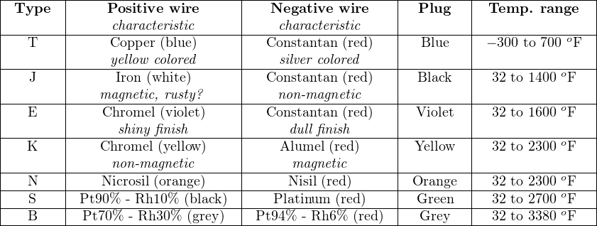
Types S and B use platinum or platinum-rhodium alloy wire, with different alloying distinguishing the positive from the negative wires. Sometimes type B is colored green and red rather than grey and red.
Note how the negative (−) wire of every thermocouple type is color-coded red. While this may seem backward to those familiar with modern electronics (where red and black usually represent the positive and negative poles of a DC power supply, respectively), bear in mind that thermocouple color codes actually pre-date electronic power supply wire coloring!
Aside from having different usable temperature ranges, these thermocouple types also differ in terms of the atmospheres they may withstand at elevated temperatures. Type J thermocouples, for instance, by virtue of the fact that one of the wire types is iron, will rapidly corrode in any oxidizing8 atmosphere. Type K thermocouples are attacked by reducing9 atmospheres as well as sulfur and cyanide. Type T thermocouples are limited in upper temperature by the oxidation of copper (a very reactive metal when hot), but stand up to both oxidizing and reducing atmospheres quite well at lower temperatures, even when wet.
One final note on the thermocouple types shown in this table is that the temperature ranges given are approximate, and vary with the intended measurement accuracy. One may have to stay within a more limited range of temperature than what is shown in this table if a certain minimum level of accuracy is desired from the thermocouple. Consult manufacturers’ data for details!
21.4.3 Connector and tip styles
In its simplest form, a thermocouple is nothing more than a pair of dissimilar-metal wires joined together. However, in industrial practice, we often must package thermocouples in a more rugged form than a bare metal junction. For instance, most industrial thermocouples are manufactured in such a way that the dissimilar-metal wires are protected from physical damage by a stainless steel or ceramic sheath, and they are often equipped with molded-plastic plugs for quick connection to and disconnection from a thermocouple-based instrument.
A photograph of a type K industrial thermocouple (approximately 20 inches in length) reveals this “sheathed” and “connectorized” construction:
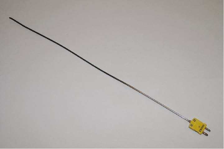
The stainless steel sheath of this particular thermocouple shows signs of discoloration from previous service in a hot process. Note the different diameters of the plug terminals. This “polarized” design makes it difficult10 to insert backward into a matching socket.
A miniature version of this same plug (designed to attach to thermocouple wire by screw terminals, rather than be molded onto the end of a sheathed assembly) is shown here, situated next to a ballpoint pen for size comparison:
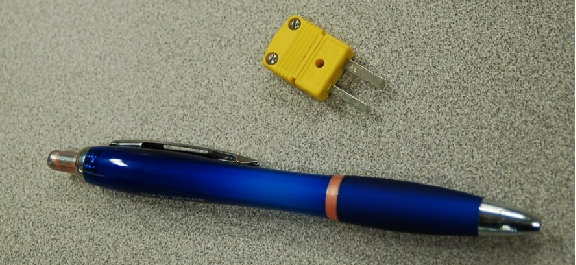
Industrial-grade thermocouples are available with this miniature style of molded plug end as an alternative to the larger (standard) plug. Miniature plug-ends are often the preferred choice for laboratory applications, while standard-sized plugs are often the preferred choice for field applications.
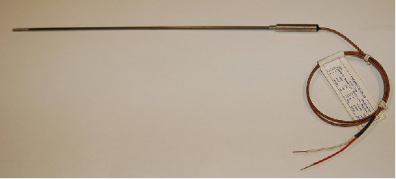
Some industrial thermocouples have no molded plug at all, but terminate simply in a pair of open wire ends. The following photograph shows a type J thermocouple of this construction:
If the electronic measuring instrument (e.g. temperature transmitter) is located near enough for the thermocouple’s wires to reach the connection terminals, no plug or socket is needed at all in the circuit. If, however, the distance between the thermocouple and measuring instrument is too far to span with the thermocouple’s own wires, a common termination technique is to attach a special terminal block and connection “head” to the top of the thermocouple allowing a pair of thermocouple extension wires to join and carry the millivoltage signal to the measuring instrument.
This next photograph shows a close-up view of such a thermocouple “head”:
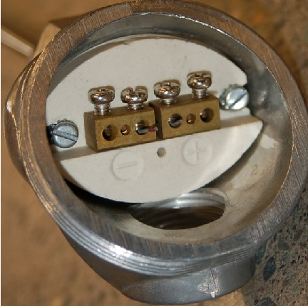
As you can see from this photograph, the screws directly press against the solid metal thermocouple wires to make a firm connection between each wire and the brass terminal block. Since the “head” attaches directly to one end of the thermocouple, the thermocouple’s wires will be trimmed just long enough to engage with the terminal screws inside the head. Both brass terminal blocks are mounted on a ceramic base, the purpose of the ceramic being to help equalize the temperatures between the two brass blocks while still maintaining electrical isolation. This assembly is sometimes referred to as an isothermal terminal block because it acts to keep all connection points at a common temperature (“iso-thermal” = “same-temperature”). A threaded cover on the head provides easy access to these connection points for installation and maintenance, while ensuring the connections are covered and protected from ambient weather conditions the rest of the time.
Thermocouple wires are most often manufactured in solid form rather than stranded form. A common mistake made with thermocouple wires is for technicians to crimp compression-style terminals (“lugs”) onto the solid wires. While this may form a usable connection at first, compression-style terminals are simply unable to maintain adequate compression when applied to solid wire of any type, thermocouple wire included. Over time, solid wires will loosen inside compression terminals leading to circuit problems. In the case of a thermocouple circuit, bad wire connections lead to a situation where the receiving instrument “thinks” the thermocouple has failed open. This situation is commonly called burnout, referring to the phenomenon where a thermocouple junction fails open from being “burned out” by excessive temperature.
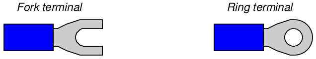
You will most often find compression terminals (improperly) applied to solid thermocouple wire tips where those wires must terminate under the head of a screw. Compression terminals are correct to use in applications where stranded wire terminates at a screw head, but not solid wire. The proper termination technique for solid wire under a screw head is to wrap the solid wire in a semi-circle and directly clamp it under the screw head.
At the other end of the thermocouple, we have a choice of tip styles. For maximum sensitivity and fastest response, the dissimilar-metal junction may be unsheathed (bare). This design, however, makes the thermocouple more fragile. Sheathed tips are typical for industrial applications, available in either grounded or ungrounded forms:
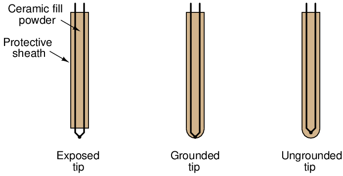
Grounded-tip thermocouples exhibit faster response times11 and greater sensitivity than ungrounded-tip thermocouples, but they are vulnerable to ground loops: circuitous paths for electric current between the conductive sheath of the thermocouple and some other point in the thermocouple circuit. In order to avoid this potentially troublesome effect, most industrial thermocouples are of the ungrounded design.
21.4.4 Manually interpreting thermocouple voltages
Recall that the amount of voltage indicated by a voltmeter connected to a thermocouple is the difference between the voltage produced by the measurement junction (the point where the two dissimilar metals join at the location we desire to sense temperature at) and the voltage produced by the reference junction (the point where the thermocouple wires join to the voltmeter wires):
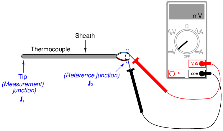

This makes thermocouples inherently differential sensing devices: they generate a measurable voltage in proportion to the difference in temperature between two locations. This inescapable fact of thermocouple circuits complicates the task of interpreting any voltage measurement obtained from a thermocouple.
In order to translate a voltage measurement produced by a voltmeter connected to a thermocouple, we must add the voltage produced by the measurement junction (V J2) to the voltage indicated by the voltmeter to find the voltage being produced by the measurement junction (V J1). In other words, we manipulate the previous equation into the following form:

We may ascertain the reference junction voltage by placing a thermometer near that junction (where the thermocouple wire attaches to the voltmeter test leads) and referencing a thermocouple table showing temperatures and corresponding voltages for that thermocouple type. Then, we may take the voltage sum for V J1 and re-reference that same table, finding the temperature value corresponding to the calculated measurement junction voltage. The National Institute of Standards and Technology (NIST) in the United States publishes tables showing junction voltages and temperatures for standardized thermocouple types. While it is possible to mathematically model a thermocouple junction’s voltage in the same way we may model an RTD’s resistance, the functions for thermocouples are less linear than for RTDs, and so tables are greatly preferred for practical use.
To illustrate, suppose we connected a voltmeter to a type K thermocouple and measured 14.30 millivolts. A thermometer situated near the thermocouple wire / voltmeter junction point shows an ambient temperature of 73 degrees Fahrenheit. Referencing a table of voltages for type K thermocouples (in this case, the NIST “ITS-90” reference standard), we see that a type K junction at 73 degrees Fahrenheit corresponds to 0.910 millivolts. Adding this figure to our meter measurement of 14.30 millivolts, we arrive at a sum of 15.21 millivolts for the measurement (“hot”) junction. Going back to the same table of values, we see 15.21 millivolts falls between 701 and 702 degrees Fahrenheit. Linearly interpolating between the table values (15.203 mV at 701 oF and 15.226 mV at 702 oF), we may more precisely determine the measurement junction to be 701.3 degrees Fahrenheit.
The process of manually taking voltage measurements, referencing a table of millivoltage values, performing addition, then re-referencing the same table is rather tedious. Compensation for the reference junction’s inevitable presence in the thermocouple circuit is something we must do, but it is not something that must always be done by a human being. The next subsection discusses ways to automatically compensate for the effect of the reference junction, which is the only practical alternative for continuous thermocouple-based temperature instruments.
21.4.5 Reference junction compensation
Multiple techniques exist to deal with the influence of the reference junction’s temperature12 . One technique is to physically fix the temperature of that junction at some constant value so it is always stable. This way, any changes in measured voltage must be due to changes in temperature at the measurement junction, since the reference junction has been rendered incapable of changing temperature. This may be accomplished by immersing the reference junction in a bath of ice and water, the ice/water mixture ensuring a stable temperature by means of water’s latent heat of fusion13 :
In fact, this is how thermocouple temperature/voltage tables are referenced: describing the amount of voltage produced for given temperatures at the measurement junction with the reference junction held at the freezing point of water (0 oC = 32 oF). With the reference junction maintained at the freezing point of water, and thermocouple tables referenced to that specific cold junction temperature, the voltmeter’s indication will simply and directly correspond to the temperature of measurement junction J1 at all times.
However, fixing the reference junction at the temperature of freezing water is impractical for any real thermocouple application outside of a laboratory. Instead, we need to find some other way to compensate for changes in reference junction temperature, so that we may accurately interpret the temperature of the measurement junction despite random changes in reference junction temperature.
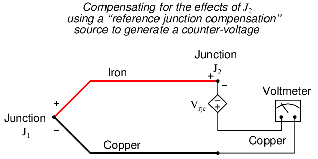
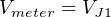
A practical way to compensate for the reference junction voltage is to include an additional voltage source within the thermocouple circuit equal in magnitude and opposite in polarity to the reference junction voltage. If this additional voltage is made continually equal to the reference junction’s potential, it will precisely counter the reference junction voltage, resulting in the full (measurement junction) voltage appearing at the measuring instrument terminals. This is called a reference junction compensation or cold junction14 compensation circuit:

In order for such a compensation strategy to work, the compensating voltage must continuously track the voltage produced by the reference junction. To do this, the compensating voltage source (V rjc in the above schematic) uses some other temperature-sensing device such as a thermistor or RTD to sense the local temperature at the terminal block where junction J2 is formed and produce a counter-voltage that is precisely equal and opposite to J2’s voltage (V rjc = V J2) at all times. Having canceled the effect of the reference junction, the voltmeter now only registers the voltage produced by the measurement junction J1:


Some instrument manufacturers sell electronic ice point modules designed to provide reference junction compensation for un-compensated instruments such as standard voltmeters. The “ice point” circuit performs the function shown by V rjc in the previous diagram: it inserts a counter-acting voltage to cancel the voltage generated by the reference junction, so that the voltmeter only “sees” the measurement junction’s voltage. This compensating voltage is maintained at the proper value according to the terminal temperature where the thermocouple wires connect to the ice point module, sensed by a thermistor or RTD:
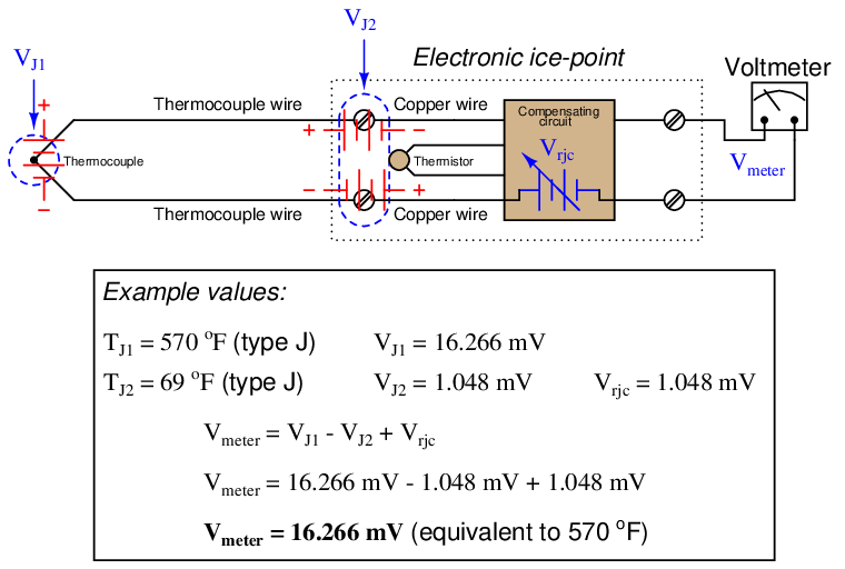
In this example, we see the measurement junction (J1) at a temperature of 570 degrees Fahrenheit, generating a voltage of 16.266 millivolts. If this thermocouple were directly connected to the meter, the meter would only register 15.218 millivolts, because the reference junction (J2, at 69 degrees Fahrenheit) opposes with its own voltage of 1.048 millivolts. With the ice point compensation circuit installed, however, the 1.048 millivolts of the reference junction is canceled by the ice point circuit’s equal-and-opposite 1.048 millivolt source. This allows the full 16.266 millivolt signal from the measurement junction reach the voltmeter where it may be read and correlated to temperature by a type J thermocouple table.
At first it may seem pointless to go through the trouble of building a reference junction compensation (ice point) circuit, when doing so requires the use of some other temperature-sensing element such as a thermistor or RTD. After all, why bother to do this just to be able to use a thermocouple to accurately measure temperature, when we could simply use this “other” device to directly measure the process temperature? In other words, isn’t the usefulness of a thermocouple invalidated if we must rely on some other type of electrical temperature sensor just to compensate for an idiosyncrasy of the thermocouple?
The answer to this very good question is that thermocouples enjoy certain advantages over these other sensor types. Thermocouples are extremely rugged and have far greater temperature-measurement ranges than thermistors, RTDs, and other primary sensing elements. However, if the application does not demand extreme ruggedness or large measurement ranges, a thermistor or RTD is most likely the better choice!
21.4.6 Law of Intermediate Metals
It is crucial to realize that the phenomenon of a “reference junction” is an inevitable effect of having to close the electric circuit loop in a circuit made of dissimilar metals. This is true regardless of the number of metals involved. In the last example, only two metals were involved: iron and copper. This formed one iron-copper junction (J1) at the measurement end and one iron-copper junction (J2) at the indicator end. Recall that the copper-copper junction J3 was of no consequence because its identical metallic composition generates no thermal voltage:
But what about more complex thermocouple circuits, involving more than two wire types? How do we define what a “reference junction” is, or how it behaves, when we have more than two dissimilar-metal junctions in the same circuit? Take for instance this example of a type J thermocouple:
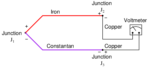
Here we have three voltage-generating junctions: J1 of iron and constantan, J2 of iron and copper, and J3 of copper and constantan15 . Upon first inspection it would seem we have a much more complex situation than we did with just two metals (iron and copper), but fortunately the situation is just as simple as it was before provided the temperatures of J2 and J3 are equal, which will be true if those two junctions are located very near each other (at the voltmeter).
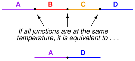
A principle of thermo-electric circuits called the Law of Intermediate Metals helps us see this clearly. According to this law, intermediate metals in a series of junctions are of no consequence to the overall (net) voltage so long as those intermediate junctions are all at the same temperature. Representing this pictorially, the net effect of having four different metals (A, B, C, and D) joined together in series is the same as just having the first and last metal in that series (A and D) joined with one junction, if all intermediate junctions are at the same temperature:
A simple proof of the Law of Intermediate Metals may be built upon the Law of Energy Conservation, one of the most fundamental principles in all of physics. Consider what would happen if we were to join the series of dissimilar metal wires shown above into a continuous loop:
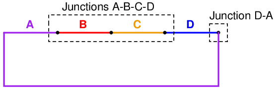
In this diagram we see that the wire made of metal “A” connects to a string of metal junctions formed by metals “B”, “C”, and “D”. If all these dissimilar metal junctions are at the same temperature, there will be no difference of temperature anywhere in the circuit to drive a current, and we would therefore expect the current in this circuit to be zero. This is in accordance with the Law of Energy Conservation, which forbids the passage of electric current through resistive wire without some motive power source driving it. Thus, based on the premise that energy must be conserved (i.e. that an electric current cannot flow through any resistance without a power source), we must conclude that the net effect of all those series-connected metal junctions at the same temperature must be zero. In other words, junctions A-B, B-C, C-D, and D-A all at the same temperature and connected in series must generate zero voltage, as if those junctions were all reduced to a single A-A junction which of course cannot produce any electromotive force (voltage) because it is not comprised of dissimilar metals. If the Law of Intermediate Metals were untrue, it would mean that the junctions A-B-C-D were not equivalent to the single junction A-D, which would mean they would produce a different voltage than the D-A junction at the right-hand end of this circuit (while at the same temperature), and therefore this circuit would produce some net voltage to drive a current continuously through resistive wire in violation of the Law of Energy Conservation. Since we know the Law of Energy Conservation to be well-founded (and we can also build such dissimilar metal loop circuits and empirically determine their currents to be zero), we may rest assured that the Law of Intermediate Metals is true.
In our type J thermocouple circuit where iron and constantan both join to copper, we see copper as an intermediate metal between junctions J2 and J3. Being located next to each other on the indicating instrument, identical temperature is a reasonable assumption for J2 and J3, so we may invoke the Law of Intermediate Metals and simply treat junctions J2 and J3 as a single iron-constantan reference junction. In other words, the Law of Intermediate Metals tells us we can treat the following two circuits identically:
The practical importance of this Law is that we can always treat the reference junction(s) as a single junction made from the same two metal types as the measurement junction, so long as all dissimilar metal junctions at the reference location are at the same temperature.
This fact is extremely important in the age of semiconductor circuitry, where the connection of a thermocouple to an electronic amplifier involves a long series of dissimilar-material junctions. Here we see a multitude of reference junctions, formed by the necessary connections from thermocouple wire to the silicon substrate inside the amplifier chip:
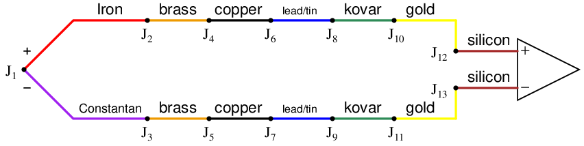
Here we see the metals of the thermocouple wire (type J – iron and constantan) joining to a pair of brass terminal screws, which in turn join to copper traces on a printed circuit board, which join to lead/tin solder, which join to thin wires made of Kovar, which terminate at gold traces on the silicon chip, which are bonded to the silicon itself.
It should be obvious that each complementary junction pair in this series loop cancel each other if each pair is at the same temperature (e.g. gold-silicon junction J12 cancels with silicon-gold junction J13 because they generate the exact same amount of voltage with opposing polarities; Kovar-gold junction J10 cancels with gold-Kovar junction J11 for the same reason; etc.). The Law of Intermediate Metals goes one step further by telling us junctions J2 through J13 taken together in series are of the same effect as a single reference junction of iron and constantan. Automatic reference junction compensation is as simple as counter-acting the voltage produced by this equivalent iron-constantan junction at whatever temperature junctions J2 through J13 happen to be at.
21.4.7 Software compensation
Previously, it was suggested that automatic compensation could be accomplished by intentionally inserting a temperature-dependent voltage source in series with the circuit, oriented in such a way as to oppose the reference junction’s voltage:

If the series voltage source V rjc is exactly equal in magnitude to the reference junction’s voltage (V J2), those two terms cancel out of the equation and lead to the voltmeter measuring only the voltage of the measurement junction J1:
This technique is known as hardware compensation, and is employed in analog thermocouple temperature transmitter designs. Previously we saw an example of this called an ice point, the purpose of which was to electrically counter the reference junction voltage to render that junction’s voltage inconsequential as though that junction were immersed in a bath of ice-water.
A modern technique for reference junction compensation more suitable to digital transmitter designs is called software compensation:
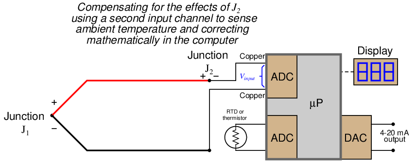
Instead of canceling the effect of the reference junction electrically, we cancel the effect arithmetically inside the microprocessor-based transmitter. In other words, we let the receiving analog-digital converter circuit see the difference in voltage between the measurement and reference junctions (V input = V J1 −V J2), but then after digitizing this voltage measurement we have the microprocessor add the equivalent voltage value corresponding to the ambient temperature sensed by the RTD or thermistor (V rjc):


Since we know the calculated value of V rjc should be equal to the real reference junction voltage (V J2), the result of this digital addition should be a compensated total equal only to the measurement junction voltage V J1:


A block diagram of a thermocouple temperature transmitter with software compensation appears here:
Perhaps the greatest advantage of software compensation is the flexibility to easily switch between different thermocouple types with no hardware modification. So long as the microprocessor memory is programmed with look-up tables relating voltage values to temperature values, it may accurately measure (and compensate for the reference junction of) any thermocouple type. Hardware-based compensation schemes (e.g. an analog “ice point” circuit) require re-wiring or replacement to accommodate different thermocouple types, since each ice-point circuit is built to generate a compensating voltage for a specific type of thermocouple.
21.4.8 Extension wire
In every thermocouple circuit there must be both a measurement junction and a reference junction: this is an inevitable consequence of forming a complete circuit (loop) using dissimilar-metal wires. As we already know, the voltage received by the measuring instrument from a thermocouple will be the difference between the voltages produced by the measurement and reference junctions. Since the purpose of most temperature instruments is to accurately measure temperature at a specific location, the effects of the reference junction’s voltage must be “compensated” for by some means, either a special circuit designed to add an additional canceling voltage or by a software algorithm to digitally cancel the reference junction’s effect.
In order for reference junction compensation to be effective, the compensation mechanism must “know” the temperature of the reference junction. This fact is so obvious, it hardly requires mentioning. However, what is not so obvious is how easily this compensation may be unintentionally defeated simply by installing a different type of wire in a thermocouple circuit.
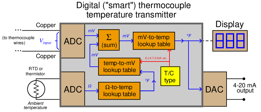
To illustrate, let us examine a simple type K thermocouple installation, where the thermocouple connects directly to a panel-mounted temperature indicator by long wires:
Like all modern thermocouple instruments, the panel-mounted indicator contains its own internal reference junction compensation, so that it is able to compensate for the temperature of the reference junction formed at its connection terminals, where the internal (copper) wires of the indicator join to the chromel and alumel wires of the thermocouple. The indicator senses this junction temperature using a small thermistor thermally bonded to the connection terminals.
Now let us consider the same thermocouple installation with a length of copper cable (two wires) joining the field-mounted thermocouple to the panel-mounted indicator:
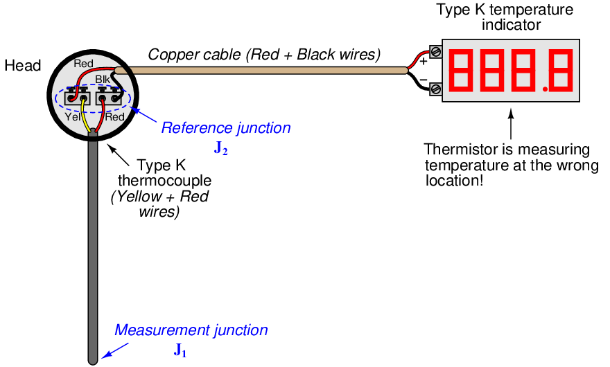
Even though nothing has changed in the thermocouple circuit except for the type of wires joining the thermocouple to the indicator, the reference junction has completely shifted position. What used to be a reference junction (at the indicator’s terminals) is no longer, because now we have copper wires joining to copper wires. Where there is no dissimilarity of metals, there can be no thermoelectric potential. At the thermocouple’s connection “head,” however we now have a joining of chromel and alumel wires to copper wires, thus forming a reference junction in a new location at the thermocouple head. What is worse, this new location is likely to be at a different temperature than the panel-mounted indicator, which means the indicator’s reference junction compensation will be compensating for the wrong temperature.
The only practical way to avoid this problem is to keep the reference junction where it belongs: at the terminals of the panel-mounted instrument where the ambient temperature is measured and the reference junction’s effects accurately compensated. If we must install “extension” wire to join a thermocouple to a remotely-located instrument, that wire must be of a type that does not form another dissimilar-metal junction at the thermocouple head, but will form one at the receiving instrument.
An obvious approach is to simply use thermocouple wire of the same type as the installed thermocouple to join the thermocouple to the indicator. For our hypothetical type K thermocouple, this means a type K cable installed between the thermocouple head and the panel-mounted indicator:
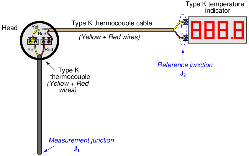
With chromel joining to chromel and alumel joining to alumel at the head, no dissimilar-metal junctions are created at the thermocouple. However, with chromel and alumel joining to copper at the indicator (again), the reference junction has been re-located to its rightful place. This means the thermocouple head’s temperature will have no effect on the performance of this measurement system, and the indicator will be able to properly compensate for any ambient temperature changes at the panel as it was designed to do. The only problem with this approach is the potential expense of thermocouple-grade cable. This is especially true with some types of thermocouples, where the metals used are somewhat exotic (e.g. types R, S, and B).
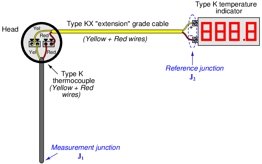
A more economical alternative, however, is to use something called extension-grade wire to make the connection between the thermocouple and the receiving instrument. “Extension-grade” thermocouple wire is made less expensive than full “thermocouple-grade” wire by choosing metal alloys similar in thermo-electrical characteristics to the real thermocouple wires within modest temperature ranges. So long as the temperatures at the thermocouple head and receiving instrument terminals don’t get too hot or too cold, the extension wire metals joining to the thermocouple wires and joining to the instrument’s copper wires need not be precisely identical to the true thermocouple wire alloys. This allows for a wider selection of metal types, some of which are substantially less expensive than the measurement-grade thermocouple alloys. Also, extension-grade wire may use insulation with a narrower temperature rating than thermocouple-grade wire, reducing cost even further.
An interesting historical reference to the use of extension-grade wire appears in Charles Robert Darling’s 1911 text Pyrometry – A Practical Treatise on the Measurement of High Temperatures. On page 61, Darling describes “compensating leads” marketed under the brand-name of Peake designed to be used with platinum-alloy thermocouples. These “compensating” wires were made of two different copper-nickel alloys, each copper-nickel alloy matched with the respective thermocouple metal (in this case, pure platinum and a 90%-10% platinum-iridium alloy) to generate an equal and opposite millivoltage at any reasonable temperature found at the thermocouple head. Thus, the only reference junction in the thermocouple circuit is where these copper-nickel extension wires joined with the indicating instrument, rather than being located at the thermocouple head as it would be if simple copper extension wires were employed. With platinum being such an expensive metal (both then and now!), the cost savings realized by being able to use cheaper extension wire to connect the platinum thermocouple to a distant receiving instrument is significant.
Extension-grade cable is denoted by a letter “X” following the thermocouple letter. For our hypothetical type K thermocouple system, this would mean type “KX” extension cable:
Thermocouple extension cable also differs from thermocouple-grade (measurement) cable in the coloring of its outer jacket. Whereas thermocouple-grade cable is typically16 brown in exterior color, extension-grade cable is usually colored17 to match the thermocouple plug (yellow for type K, black for type J, blue for type T, etc.).
21.4.9 Side-effects of reference junction compensation
Reference junction compensation is a necessary part of any precision thermocouple circuit, due to the inescapable fact of the reference junction’s existence. When you form a complete circuit of dissimilar metals, you will form both a measurement junction and a reference junction, with those two junctions’ polarities opposed to one another. This is why reference junction compensation – whether it takes the form of a hardware circuit or an algorithm in software – must exist within every precision thermocouple instrument.
The presence of reference junction compensation in every precision thermocouple instrument results in an interesting phenomenon: if you directly short-circuit the thermocouple input terminals of such an instrument, it will always register ambient temperature, regardless of the thermocouple type the instrument is built or configured for. This behavior may be illustrated by example, first showing a normal operating temperature measurement system and then with that same system short-circuited. Here we see a temperature indicator receiving a 4-20 mA current signal from a temperature transmitter, which is receiving a millivoltage signal from a type “K” thermocouple sensing a process temperature of 780 degrees Fahrenheit:
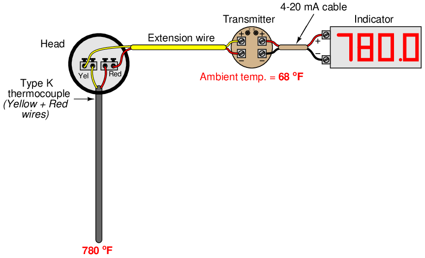
The transmitter’s internal reference junction compensation feature compensates for the ambient temperature of 68 degrees Fahrenheit. If the ambient temperature rises or falls, the compensation will automatically adjust for the change in reference junction potential, such that the output will still register the process (measurement junction) temperature of 780 degrees F. This is what the reference junction compensation is designed to do.
Now, we disconnect the thermocouple from the temperature transmitter and short-circuit the transmitter’s input:
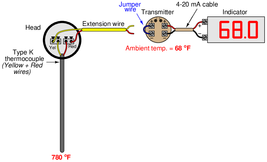
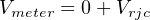
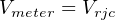
With the input short-circuited, the transmitter “sees” no voltage at all from the thermocouple circuit. There is no measurement junction nor a reference junction to compensate for, just a piece of wire making both input terminals electrically common. This means the reference junction compensation inside the transmitter no longer performs a useful function. However, the transmitter does not “know” it is no longer connected to the thermocouple, so the compensation keeps on working even though it has nothing to compensate for. Recall the voltage equation relating measurement, reference, and compensation voltages in a hardware-compensated thermocouple instrument:

Disconnecting the thermocouple wire and connecting a shorting jumper to the instrument eliminates the V J1 and V J2 terms, leaving only the compensation voltage to be read by the meter18 :
This is why the instrument registers the equivalent temperature created by the reference junction compensation feature: this is the only signal it “sees” with its input short-circuited. This phenomenon is true regardless of which thermocouple type the instrument is configured for, which makes it a convenient “quick test” of instrument function in the field. If a technician short-circuits the input terminals of any thermocouple instrument, it should respond as though it is sensing ambient temperature.
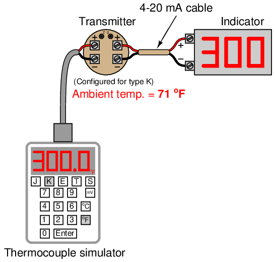
While this interesting trait is a somewhat useful side-effect of reference junction compensation in thermocouple instruments, there are other effects that are not quite so useful. The presence of reference junction compensation becomes quite troublesome, for example, if one tries to simulate a thermocouple using a precision millivoltage source. Simply setting the millivoltage source to the value corresponding to the desired (simulation) temperature given in a thermocouple table will yield an incorrect result for any ambient temperature other than the freezing point of water!
Suppose, for example, a technician wished to simulate a type K thermocouple at 300 degrees Fahrenheit by setting a millivolt source to 6.094 millivolts (the voltage corresponding to 300 oF for type K thermocouples according to the ITS-90 standard). Connecting the millivolt source to the instrument will not result in an instrument response appropriate for 300 degrees F:
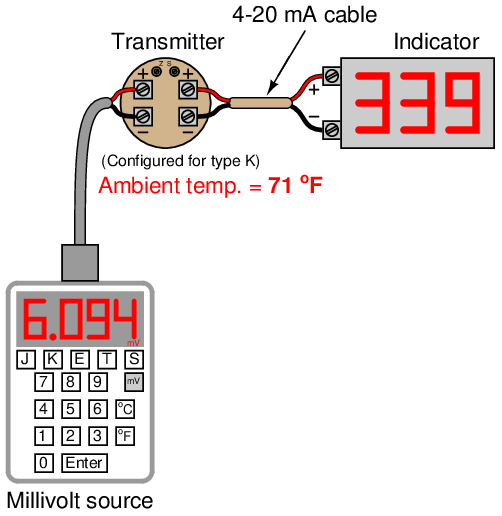
Instead, the instrument registers 339 degrees because its internal reference junction compensation feature is still active, compensating for a reference junction voltage that no longer exists. The millivolt source’s output of 6.094 mV gets added to the compensation voltage (inside the transmitter) of 0.865 mV – the necessary millivolt value to compensate for a type K reference junction at 71 oF – with the result being a larger millivoltage (6.959 mV) interpreted by the transmitter as a temperature of 339 oF.
One way to use a millivoltage source to simulate a desired temperature is for the instrument technician to “out-think” the transmitter’s compensation feature by specifying a millivolt signal that is offset by the amount of equivalent voltage generated by the transmitter’s compensation. In other words, instead of setting the millivolt source to a value of 6.094 mV, the technician should set the source to only 5.229 mV so the transmitter’s compensation will add 0.865 mV to this value to arrive at 6.094 mV and properly register as 300 degrees Fahrenheit:

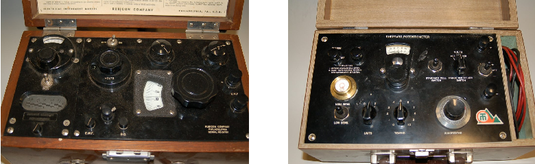
Years ago, the only suitable piece of test equipment available for generating the precise millivoltage signals necessary to calibrate thermocouple instruments was a device called a precision potentiometer. These “potentiometers” used a stable mercury cell battery (sometimes called a standard cell) as a voltage reference and a potentiometer with a calibrated knob to output low-voltage signals. Photographs of two vintage precision potentiometers are shown here:
Of course, modern thermocouple calibrators also provide direct entry of temperature and automatic compensation to “un-compensate” the transmitter such that any desired temperature may be easily simulated:
In this example, when the technician sets the calibrator for 300 oF (type K), it measures the ambient temperature and automatically subtracts 0.865 mV from the output signal, so only 5.229 mV is sent to the transmitter terminals instead of the full 6.094 mV. The transmitter’s internal reference junction compensation adds the 0.865 mV offset value (thinking it must compensate for a reference junction that in reality is not there) and “sees” a total signal voltage of 6.094 mV, interpreting this properly as 300 degrees Fahrenheit.
The following photograph shows the display of a modern thermocouple calibration device (a Fluke model 744 documenting process calibrator) being used to generate a thermocouple signal. In this particular example, the thermocouple type is set to type “S” (Platinum-Rhodium/Platinum) at a temperature of 2650 degrees Fahrenheit:
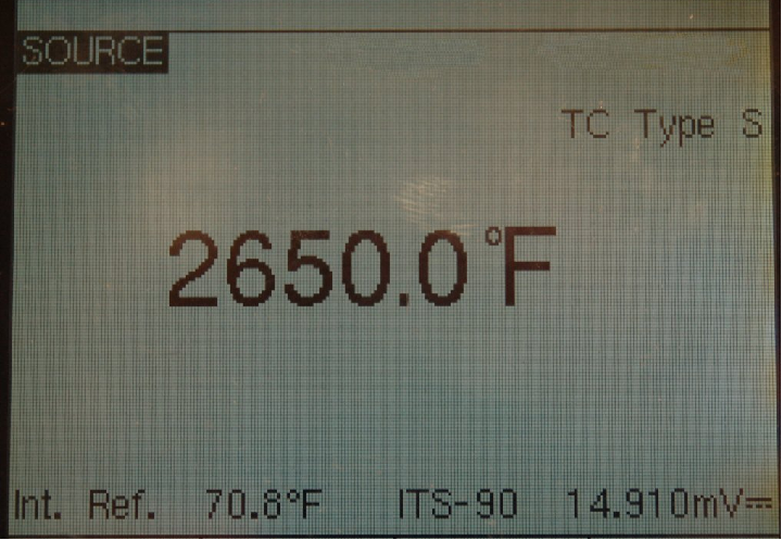
The ITS-90 thermocouple standard declares a millivoltage signal value of 15.032 mV for a type S thermocouple junction at 2650 degrees F (with a reference junction temperature of 32 degrees F). Note how the calibrator does not output 15.032 mV even though the simulated temperature has been set to 2650 degrees F. Instead, it outputs 14.910 mV, which is 0.122 mV less than 15.032 mV. This offset of 0.122 mV corresponds to the calibrator’s local temperature of 70.8 degrees F (according to the ITS-90 standard for type S thermocouples).
When the calibrator’s 14.910 mV signal reaches the thermocouple instrument being calibrated (be it an indicator, transmitter, or even a controller equipped with a type S thermocouple input), the instrument’s own internal reference junction compensation will add 0.122 mV to the received signal of 14.910 mV, “thinking” it needs to compensate for a real reference junction. The result will be a perceived measurement junction signal of 15.032 mV, which is exactly what we want the instrument to “think” it sees if our goal is to simulate connection to a real type S thermocouple at a temperature of 2650 degrees F.
21.4.10 Burnout detection
Another consideration for thermocouples is burnout detection. The most common failure mode for thermocouples is to fail open, otherwise known as “burning out.” An open thermocouple is problematic for any voltage-measuring instrument with high input impedance because the lack of a complete circuit on the input makes it possible for electrical noise from surrounding sources (power lines, electric motors, variable-frequency motor drives) to be detected by the instrument and falsely interpreted as a wildly varying temperature.
For this reason it is prudent to design into the thermocouple instrument some provision for generating a consistent state in the absence of a complete circuit. This is called the burnout mode of a thermocouple instrument. A simple thermocouple circuit equipped with burnout detection is shown in this diagram:
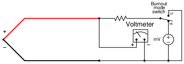
The resistor in this circuit provides a connection to a stable voltage19 in the event of an open thermocouple. It is sized in the mega-ohm range to minimize its effect during normal operation when the thermocouple circuit is complete. Only when the thermocouple fails open will the miniscule current through the resistor have any substantial effect on the voltmeter’s indication. The SPDT switch provides a selectable burnout mode: in the event of a burnt-out thermocouple, we can configure the meter to either read high temperature (sourced by the instrument’s internal milli-voltage source) or low temperature (grounded), depending on what failure mode we deem safest20 for the application.