
A 4 to 20 mA current signal represents some signal along a 0 to 100 percent scale. Usually, this scale is linear as shown by this graph:
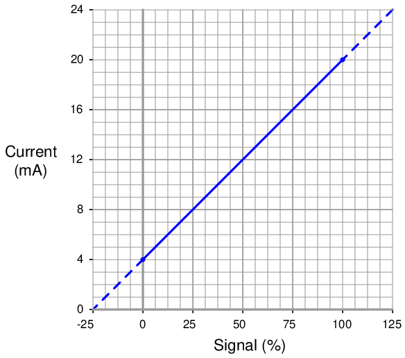
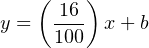
Being a linear function, we may use the standard slope-intercept linear equation to relate signal percentage to current values:

Where,
y = Output from instrument
x = Input to instrument
m = Slope
b = y-intercept point (i.e. the live zero of the instrument’s range)
Once we determine suitable values for m and b, we may then use this linear equation to predict any value for y given x, and vice-versa. This is very useful for predicting the 4-20 mA signal output of a process transmitter, or the expected stem position of a 4-20 mA controlled valve, or any other correspondence between a 4-20 mA signal and some physical variable.
Before we may use this equation for any practical purpose, we must determine the slope (m) and intercept (b) values appropriate for the instrument we wish to apply the equation to. Next, we will see some examples of how to do this.
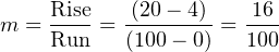
For the linear function shown, we may determine the slope value (m) by dividing the line’s rise by its run. Two sets of convenient points we may use in calculating rise over run are 4 and 20 milliamps (for the rise), and 0 and 100 percent (for the run):
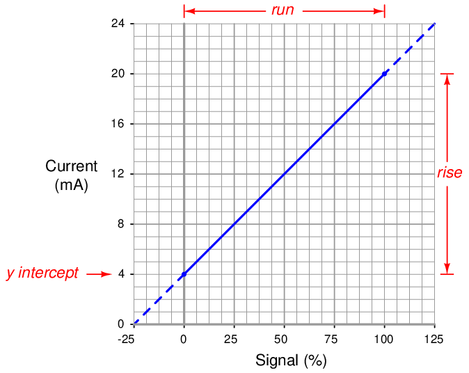
To calculate the y-intercept (b), all we need to do is solve for b at some known coordinate pair of x and y. Again, we find convenient points3 for this task at 0 percent and 4 milliamps:
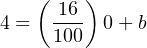


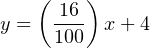
Now we have a complete formula for converting a percentage value into a milliamp value:
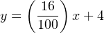
We may now use this formula to calculate how many milliamps represent any given percentage of signal. For example, suppose we needed to convert a percentage of 34.7% into a corresponding 4-20 mA current. We would do so like this:
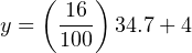
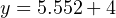

Thus, 34.7% is equivalent to 9.552 milliamps in a 4-20 mA signal range.
The slope-intercept formula for linear functions may be applied to any linear instrument, as illustrated in the following examples.
13.2.1 Example calculation: controller output to valve
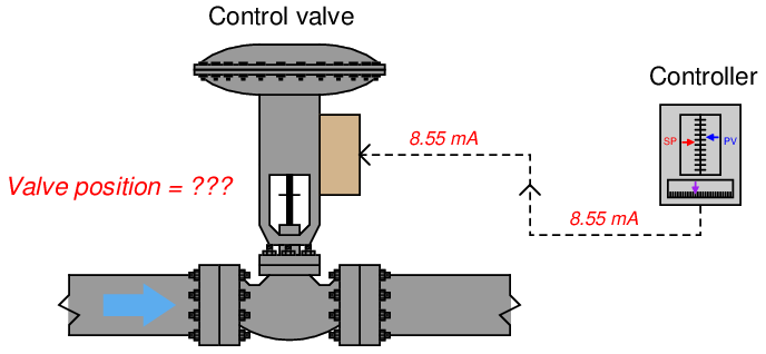
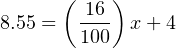
An electronic loop controller outputs a signal of 8.55 mA to a direct-responding control valve (where 4 mA is shut and 20 mA is wide open). How far open should the control valve be at this MV signal level?
To solve for percentage of stem travel (x) at 8.55 milliamps of signal current (y), we may use the linear equation developed previously to predict current in milliamps (y) from signal value in percent (x):
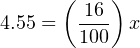

Therefore, we should expect the valve to be 28.4% open at an applied MV signal of 8.55 milliamps.
13.2.2 Example calculation: flow transmitter
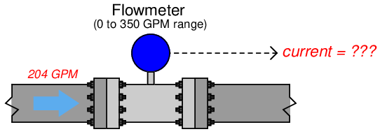
A flow transmitter is ranged 0 to 350 gallons per minute, 4-20 mA output, direct-responding. Calculate the current signal value at a flow rate of 204 GPM.
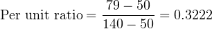
One way we could solve for the amount of signal current is to convert the flow value of 204 GPM into a ratio of the flowmeter’s full-flow value, then apply the same formula we used in the previous example relating percentage to milliamps. Converting the flow rate into a “per unit” ratio is a matter of simple division, since the flow measurement range is zero-based:
Converting a “per unit” ratio into percent merely requires multiplication by 100, since “percent” literally means “per 100”:

Next, we plug this percentage value into the formula:
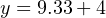

Therefore, the transmitter should output a PV signal of 13.3 mA at a flow rate of 204 GPM.
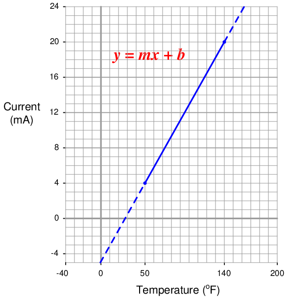
An alternative approach is to set up a linear equation specifically for this flowmeter given its measurement range (0 to 350 GPM) and output signal range (4 to 20 mA). We will begin this process by sketching a simple graph relating flow rate to current:
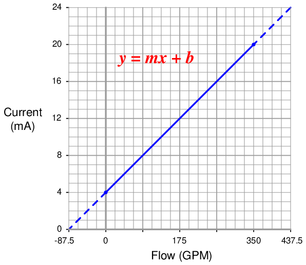
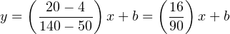
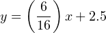
The slope (m) for this equation is rise over run, in this case 16 milliamps of rise for 350 GPM of run:
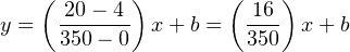
The y-intercept for this equation is 4, since the current output will be 4 milliamps at zero flow:
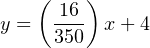
Now that the linear equation is set up for this particular flowmeter, we may plug in the 204 GPM value for x and solve for current:
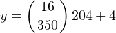


Just as before, we arrive at a current of 13.33 milliamps representing a flow rate of 204 GPM.
13.2.3 Example calculation: temperature transmitter
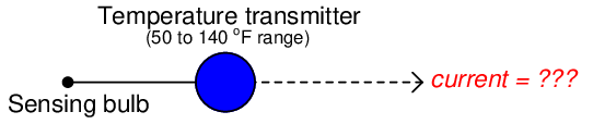
An electronic temperature transmitter is ranged 50 to 140 degrees Fahrenheit and has a 4-20 mA output signal. Calculate the current output by this transmitter if the measured temperature is 79 degrees Fahrenheit.
First, we will set up a linear equation describing this temperature transmitter’s function:
Calculating and substituting the slope (m) value for this equation, using the full rise-over-run of the linear function:
The y-intercept value will be different4 for this example than it was for previous examples, since the measurement range is not zero-based. However, the procedure for finding this value is the same – plug any corresponding x and y values into the equation and solve for b. In this case, I will use the values of 4 mA for y and 50 oF for x:

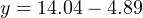
Therefore, our customized linear equation for this temperature transmitter is as follows:
At a sensed temperature of 79 oF, the transmitter’s output current will be 9.16 mA:

We may apply the same alternative method of solution to this problem as we did for the flowmeter example: first converting the process variable into a simple “per unit” ratio or percentage of measurement range, then using that percentage to calculate current in milliamps. The “tricky” aspect of this example is the fact the temperature measurement range does not begin at zero.
Converting 79 oF into a percentage of a 50-to-140 oF range requires that we first subtract the live-zero value, then divide by the span:

Next, plugging this percentage value into our standard linear equation for 4-20 mA signals:
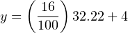

Again, we arrive at the exact same figure for transmitter output current: 9.16 milliamps at a measured temperature of 79 oF.
The choice to calculate transmitter current by first setting up a “customized” linear equation for the transmitter in question or by converting the measured value into a percentage and using a “standard” linear equation for current is arbitrary. Either method will produce accurate results, although it could be argued that the “customized equation” approach may save time if many different current values must be calculated.
Certainly, if you are programming a computer to convert a received milliamp signal value into a measurement range (such as degrees Fahrenheit), it makes more sense to have the computer evaluate a single equation rather than perform multiple steps of calculations as we do when using percentage values as an intermediate step between the input and output value calculations. Evaluating one equation rather than two saves processing time.
13.2.4 Example calculation: pH transmitter
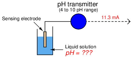
A pH transmitter has a calibrated range of 4 pH to 10 pH, with a 4-20 mA output signal. Calculate the pH sensed by the transmitter if its output signal is 11.3 mA.
First, we will set up a linear equation describing this temperature transmitter’s function:
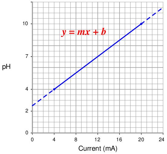
Note how we are free to set up 4-20 mA as the independent variable (x axis) and the pH as the dependent variable (y axis). We could arrange current on the y axis and the process measurement on the x axis as before, but this would force us to manipulate the linear equation to solve for x.
Calculating and substituting the slope (m) value for this equation, using the full rise-over-run of the linear function:
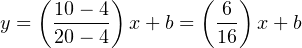
Solving for the y-intercept value using the coordinate values of 4 pH and 4 mA, we see again that this is an application where b ≠ 4 mA. This is due to the fact that the instrument’s input range (i.e. the domain of the y = mx + b function) does not begin at zero:
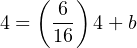


Therefore, our customized linear equation for this pH transmitter is as follows:
Calculating the corresponding pH value for an output current signal of 11.3 mA now becomes a very simple matter:
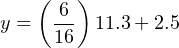
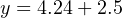

Therefore, the transmitter’s 11.3 mA output signal reflects a measured pH value of 6.74 pH.
13.2.5 Example calculation: reverse-acting I/P transducer signal
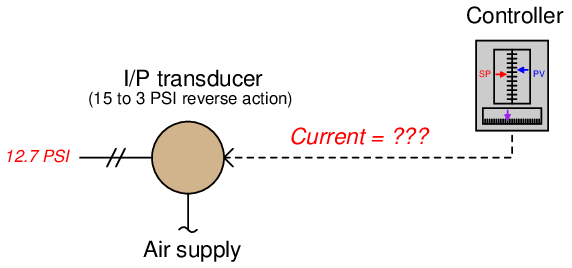
A current-to-pressure transducer is used to convert a 4-20 mA electronic signal into a 3-15 PSI pneumatic signal. This particular transducer is configured for reverse action instead of direct, meaning that its pressure output at 4 mA should be 15 PSI and its pressure output at 20 mA should be 3 PSI. Calculate the necessary current signal value to produce an output pressure of 12.7 PSI.
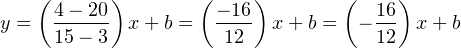
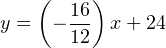
Reverse-acting instruments are still linear, and therefore still follow the slope-intercept line formula y = mx + b, albeit with a negative slope:
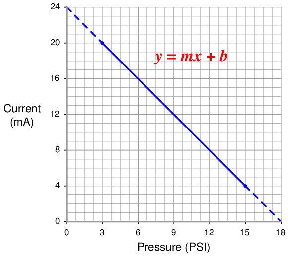
Calculating and substituting the slope (m) value for this equation, using the full rise-over-run of the linear function. Note how the “rise” is actually a “fall” from 20 milliamps down to 4 milliamps, yielding a negative value for m:
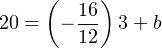
Solving for the y-intercept value using the coordinate values of 3 PSI and 20 mA:

Therefore, our customized linear equation for this I/P transducer is as follows:
Calculating the corresponding current signal for an output pressure of 12.7 PSI:
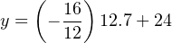

Therefore, a current signal of 7.07 mA is necessary to drive the output of this reverse-acting I/P transducer to a pressure of 12.7 PSI.
13.2.6 Example calculation: PLC analog input scaling
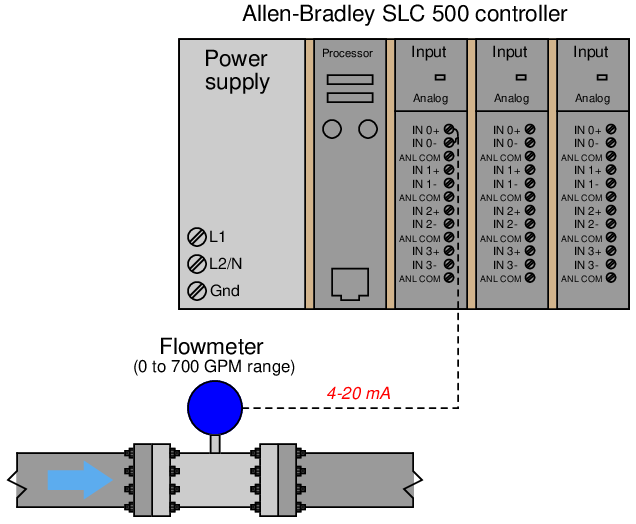
An Allen-Bradley SLC500 programmable logic controller (PLC) uses a 16-bit analog-to-digital converter in its model 1746-NI4 analog input card to convert 4-20 mA signals into digital number values ranging from 3277 (at 4 mA) to 16384 (at 20 mA). However, these raw numbers from the PLC’s analog card must be mathematically scaled inside the PLC to represent real-world units of measurement, in this case 0 to 700 GPM of flow. Formulate a scaling equation to program into the PLC so that 4 mA of current registers as 0 GPM, and 20 mA of current registers as 700 GPM.
We are already given the raw number values from the analog card’s analog-to-digital converter (ADC) circuit for 4 mA and 20 mA: 3277 and 16384, respectively. These values define the domain of our linear graph:
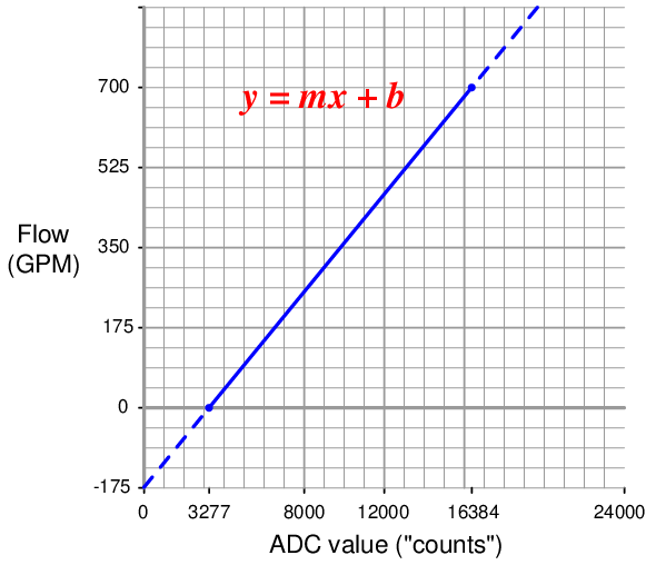
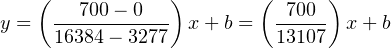
Calculating and substituting the slope (m) value for this equation, using the full rise-over-run of the linear function:
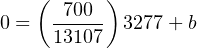
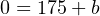
Solving for the y-intercept value using the coordinate values of 0 GPM and 3277 ADC counts:

Therefore, our PLC scaling equation for this particular flowmeter is as follows:
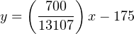
This type of scaling calculation is so common in PLC applications that Allen-Bradley has provided a special SCL (“scale”) instruction just for this purpose. Instead of “slope” (m) and “intercept” (b), the instruction prompts the human programmer to enter “rate” and “offset” values, respectively. Furthermore, the rate in Allen-Bradley’s SCL instruction is expressed as the numerator of a fraction where the denominator is fixed at 10000, allowing fractional (less than one) slope values to be specified using integer numbers. Aside from these details, the concept is exactly the same.
Expressing our slope of 700 _ 13107 as a fraction with 10000 as the denominator is a simple matter of solving for the numerator using cross-multiplication and division:


Thus, the SCL instruction would be configured as follows5
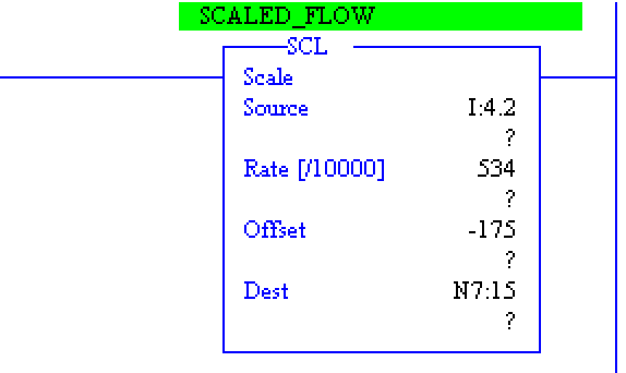
13.2.7 Graphical interpretation of signal ranges
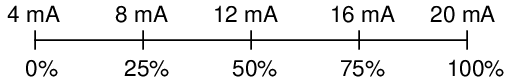
An illustration some students find helpful in understanding analog signal ranges is to consider the signal range as a length expressed on a number line. For example, the common 4-20 mA analog current signal range would appear as such:
If one were to ask the percentage corresponding to a 14.4 mA signal on a 4-20 mA range, it would be as simple as determining the length of a line segment stretching from the 4 mA mark to the 14.4 mA mark:
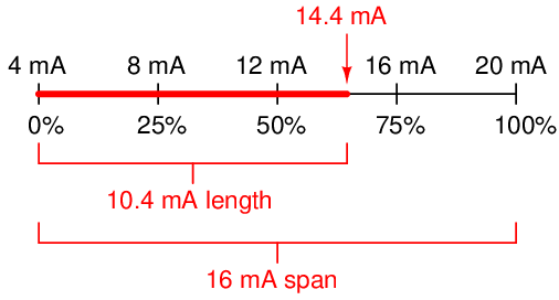
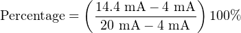
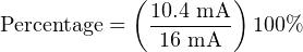
As a percentage, this thick line is 10.4 mA long (the distance between 14.4 mA and 4 mA) over a total (possible) length of 16 mA (the total span between 20 mA and 4 mA). Thus:

This same “number line” approach may be used to visualize any conversion from one analog scale to another. Consider the case of an electronic pressure transmitter calibrated to a pressure range of −5 to +25 PSI, having an (obsolete) current signal output range of 10 to 50 mA. The appropriate current signal value for an applied pressure of +12 PSI would be represented on the number line as such:
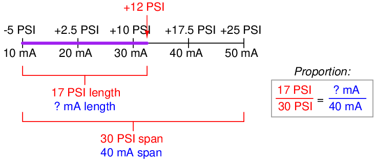
Finding the “length” of this line segment in units of milliamps is as simple as setting up a proportion between the length of the line in units of PSI over the total (span) in PSI, to the length of the line in units of mA over the total (span) in mA:
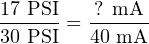
Solving for the unknown (?) current by cross-multiplication and division yields a value of 22.67 mA. Of course, this value of 22.67 mA only tells us the length of the line segment on the number line; it does not directly tell us the current signal value. To find that, we must add the “live zero” offset of 10 mA, for a final result of 32.67 mA.
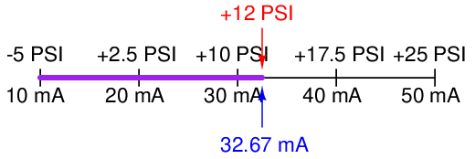
Thus, an applied pressure of +12 PSI to this transmitter should result in a 32.67 mA output signal.
13.2.8 Thinking in terms of per unit quantities
Although it is possible to generate a “custom” linear equation in the form of y = mx + b for any linear-responding instrument relating input directly to output, a more general approach may be used to relate input to output values by translating all values into (and out of) per unit quantities. A “per unit” quantity is simply a ratio between a given quantity and its maximum value. A half-full glass of water could thus be described as having a fullness of 0.5 per unit. The concept of percent (“per one hundred”) is very similar, the only difference between per unit and percent being the base value of comparison: half-full glass of water has a fullness of 0.5 per unit (i.e. 1 2 of the glass’s full capacity), which is the same thing as 50 percent (i.e. 50 on a scale of 100, with 100 representing complete fullness).
Let’s now apply this concept to a realistic 4-20 mA signal application. Suppose you were given a liquid level transmitter with an input measurement range of 15 to 85 inches and an output range of 4 to 20 milliamps, respectively, and you desired to know how many milliamps this transmitter should output at a measured liquid level of 32 inches. Both the measured level and the milliamp signal may be expressed in terms of per unit ratios, as shown by the following graphs:
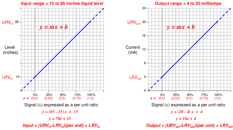
So long as we choose to express process variable and analog signal values as a per unit ratios ranging from 0 to 1, we see how m (the slope of the line) is simply equal to the span of the process variable or analog signal range, and b is simply equal to the lower-range value (LRV) of the process variable or analog signal range. The advantage of thinking in terms of “per unit” is the ability to quickly and easily write linear equations for any given range. In fact, this is so easy that we don’t even have to use a calculator to compute m in most cases, and we never have to calculate b because the LRV is explicitly given to us. The instrument’s input equation is y = 70x + 15 because the span of the 15-to-85 inch range is 70, and the LRV is 15. The instrument’s output equation is y = 16x + 4 because the span of the 4-to-20 milliamp range is 16, and the LRV is 4.
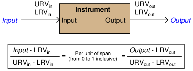
If we manipulate each of the y = mx + b equations to solve for x (per unit of span), we may express the relationship between the input and output of any linear instrument as a pair of fractions with the per unit value serving as the proportional link between input and output:
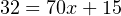
The question remains, how do we apply these equations to our example problem: calculating the milliamp value corresponding to a liquid level of 32 inches for this instrument? The answer to this question is that we must perform a two-step calculation: first, convert 32 inches into a per unit ratio, then convert that per unit ratio into a milliamp value.
First, the conversion of inches into a per unit ratio, knowing that 32 is the value of y and we need to solve for x:

Next, converting this per unit ratio into a corresponding milliamp value, knowing that y will now be the current signal value using m and b constants appropriate for the 4-20 milliamp range:
Instead of deriving a single custom y = mx + b equation directly relating input (inches) to output (milliamps) for every instrument we encounter, we may use two simple and generic linear equations to do the calculation in two steps with “per unit” being the intermediate result. Expressed in general form, our linear equation is:


Thus, to find the per unit ratio we simply take the value given to us, subtract the LRV of its range, and divide by the span of its range. To find the corresponding value we take this per unit ratio, multiply by the span of the other range, and then add the LRV of the other range.
Example: Given a pressure transmitter with a measurement range of 150 to 400 PSI and a signal range of 4 to 20 milliamps, calculate the applied pressure corresponding to a signal of 10.6 milliamps.
Solution: Take 10.6 milliamps and subtract the LRV (4 milliamps), then divide by the span (16 milliamps) to arrive at 41.25% (0.4125 per unit). Take this number and multiply by the span of the pressure range (400 PSI − 150 PSI, or 250 PSI) and lastly add the LRV of the pressure range (150 PSI) to arrive at a final answer of 253.125 PSI.
Example: Given a temperature transmitter with a measurement range of −88 degrees to +145 degrees and a signal range of 4 to 20 milliamps, calculate the proper signal output at an applied temperature of +41 degrees.
Solution: Take 41 degrees and subtract the LRV (−88 degrees) which is the same as adding 88 to 41, then divide by the span (145 degrees − (−88) degrees, or 233 degrees) to arrive at 55.36% (0.5536 per unit). Take this number and multiply by the span of the current signal range (16 milliamps) and lastly add the LRV of the current signal range (4 milliamps) to arrive at a final answer of 12.86 milliamps.
Example: Given a pH transmitter with a measurement range of 3 pH to 11 pH and a signal range of 4 to 20 milliamps, calculate the proper signal output at 9.32 pH.
Solution: Take 9.32 pH and subtract the LRV (3 pH), then divide by the span (11 pH − 3 pH, or 8 pH) to arrive at 79% (0.79 per unit). Take this number and multiply by the span of the current signal range (16 milliamps) and lastly add the LRV of the current signal range (4 milliamps) to arrive at a final answer of 16.64 milliamps.