
Whenever there is a mismatch of impedance between transmission line and load, reflections will occur. If the incident signal is a continuous AC waveform, these reflections will mix with more of the oncoming incident waveform to produce stationary waveforms called standing waves.
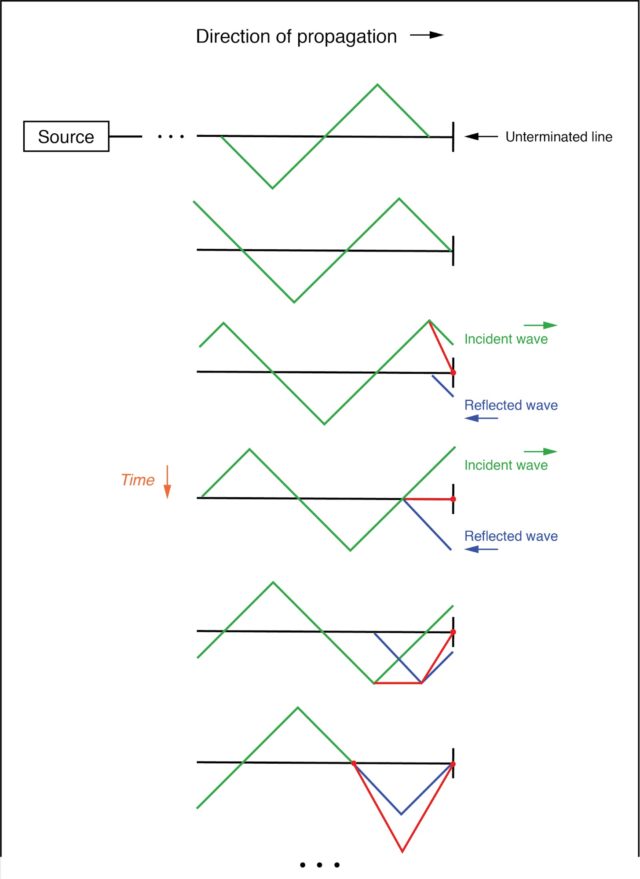
The following illustration shows how a triangle-shaped incident waveform turns into a mirror-image reflection upon reaching the line’s unterminated end. The transmission line in this illustrative sequence is shown as a single, thick line rather than a pair of wires, for simplicity’s sake. The incident wave is shown traveling from left to right, while the reflected wave travels from right to left: (Figure below)
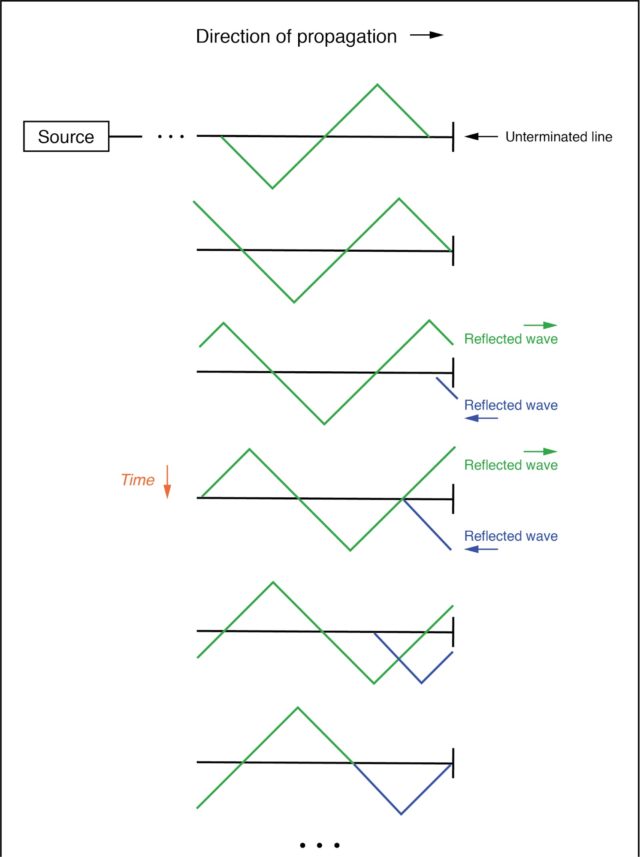
Incident wave reflects off end of unterminated transmission line.
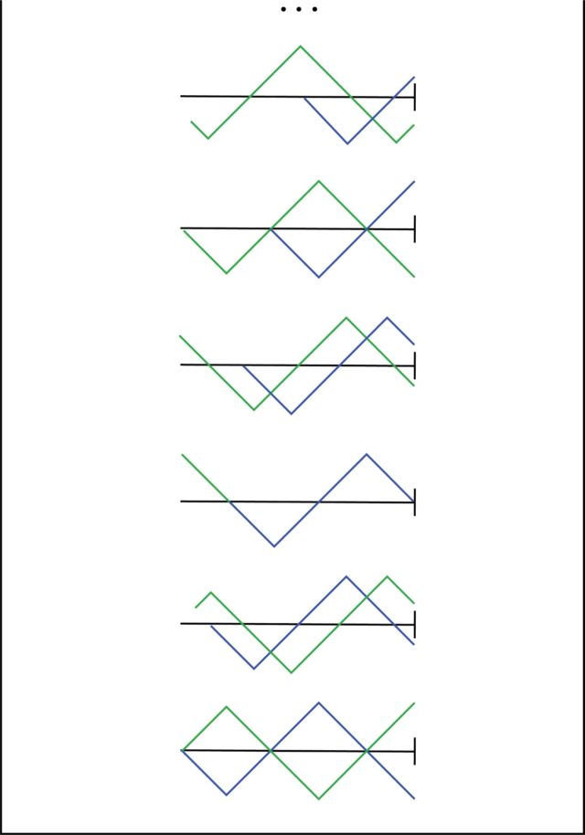
If we add the two waveforms together, we find that a third, stationary waveform is created along the line’s length: (Figure below)
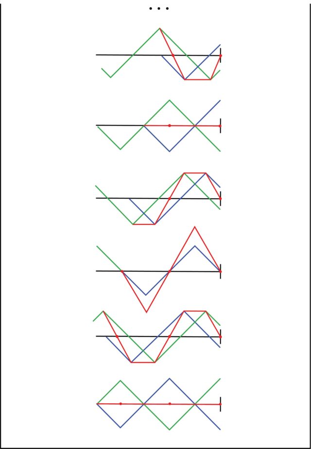
The sum of the incident and reflected waves is a stationary wave.
This third, “standing” wave, in fact, represents the only voltage along the line, being the representative sum of incident and reflected voltage waves. It oscillates in instantaneous magnitude, but does not propagate down the cable’s length like the incident or reflected waveforms causing it. Note the dots along the line length marking the “zero” points of the standing wave (where the incident and reflected waves cancel each other), and how those points never change position: (Figure below)
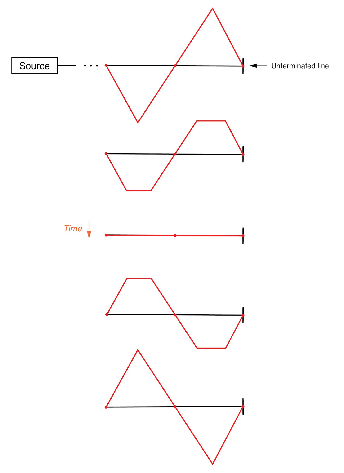
The standing wave does not propgate along the transmission line.
Cases Where a Standing Wave is Produced
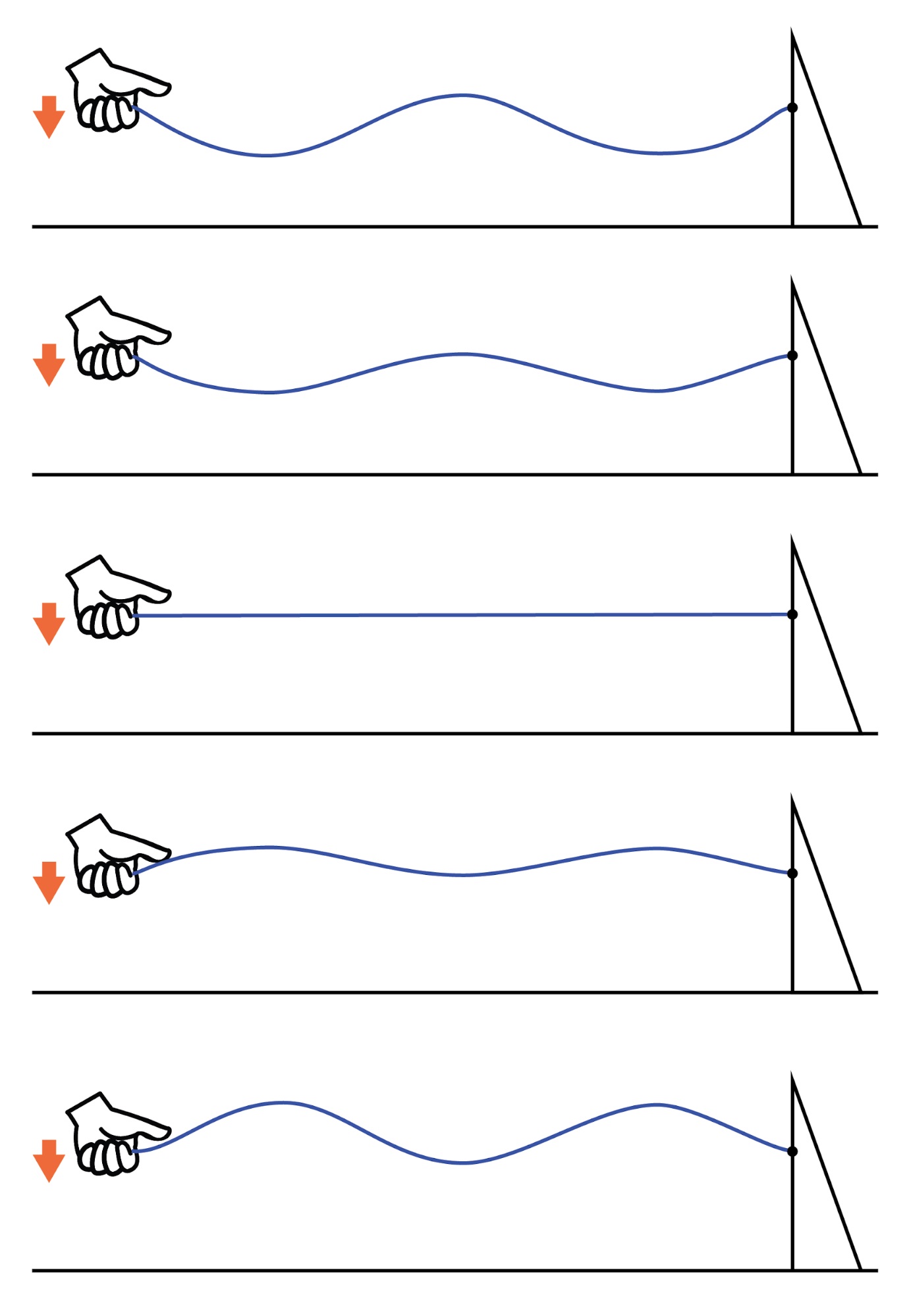
Standing waves are quite abundant in the physical world. Consider a string or rope, shaken at one end, and tied down at the other (only one half-cycle of hand motion shown, moving downward): (Figure below)
Standing waves on a rope.
Both the nodes (points of little or no vibration) and the antinodes (points of maximum vibration) remain fixed along the length of the string or rope. The effect is most pronounced when the free end is shaken at just the right frequency. Plucked strings exhibit the same “standing wave” behavior, with “nodes” of maximum and minimum vibration along their length. The major difference between a plucked string and a shaken string is that the plucked string supplies its own “correct” frequency of vibration to maximize the standing-wave effect: (Figure below)

Standing waves on a plucked string.
Wind blowing across an open-ended tube also produces standing waves; this time, the waves are vibrations of air molecules (sound) within the tube rather than vibrations of a solid object. Whether the standing wave terminates in a node (minimum amplitude) or an antinode (maximum amplitude) depends on whether the other end of the tube is open or closed: (Figure below)

Standing sound waves in open ended tubes.
A closed tube end must be a wave node, while an open tube end must be an antinode. By analogy, the anchored end of a vibrating string must be a node, while the free end (if there is any) must be an antinode.
Progression of Harmonics of Resonant Frequencies
Note how there is more than one wavelength suitable for producing standing waves of vibrating air within a tube that precisely match the tube’s end points. This is true for all standing-wave systems: standing waves will resonate with the system for any frequency (wavelength) correlating to the node/antinode points of the system. Another way of saying this is that there are multiple resonant frequencies for any system supporting standing waves.
All higher frequencies are integer-multiples of the lowest (fundamental) frequency for the system. The sequential progression of harmonics from one resonant frequency to the next defines the overtone frequencies for the system: (Figure below)
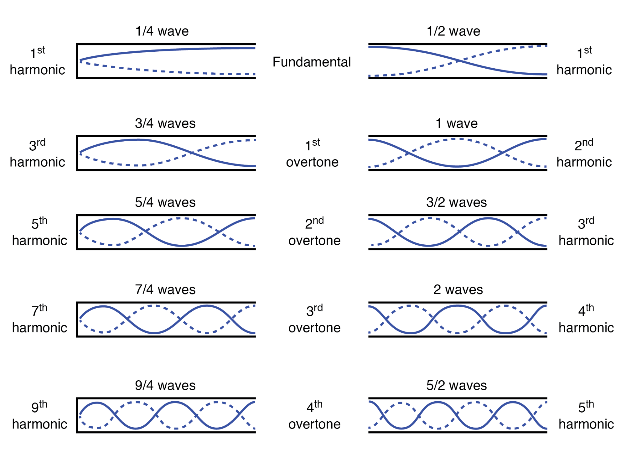
Harmonics (overtones) in open ended pipes
The actual frequencies (measured in Hertz) for any of these harmonics or overtones depends on the physical length of the tube and the waves’ propagation velocity, which is the speed of sound in air.
Simulating a Transmission Line Resonance using SPICE
Because transmission lines support standing waves, and force these waves to possess nodes and antinodes according to the type of termination impedance at the load end, they also exhibit resonance at frequencies determined by physical length and propagation velocity. Transmission line resonance, though, is a bit more complex than resonance of strings or of air in tubes, because we must consider both voltage waves and current waves.
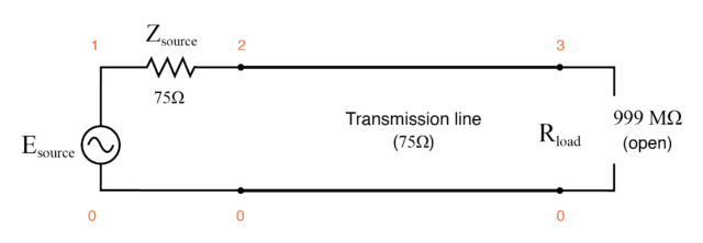
This complexity is made easier to understand by way of computer simulation. To begin, let’s examine a perfectly matched source, transmission line, and load. All components have an impedance of 75 Ω: (Figure below)
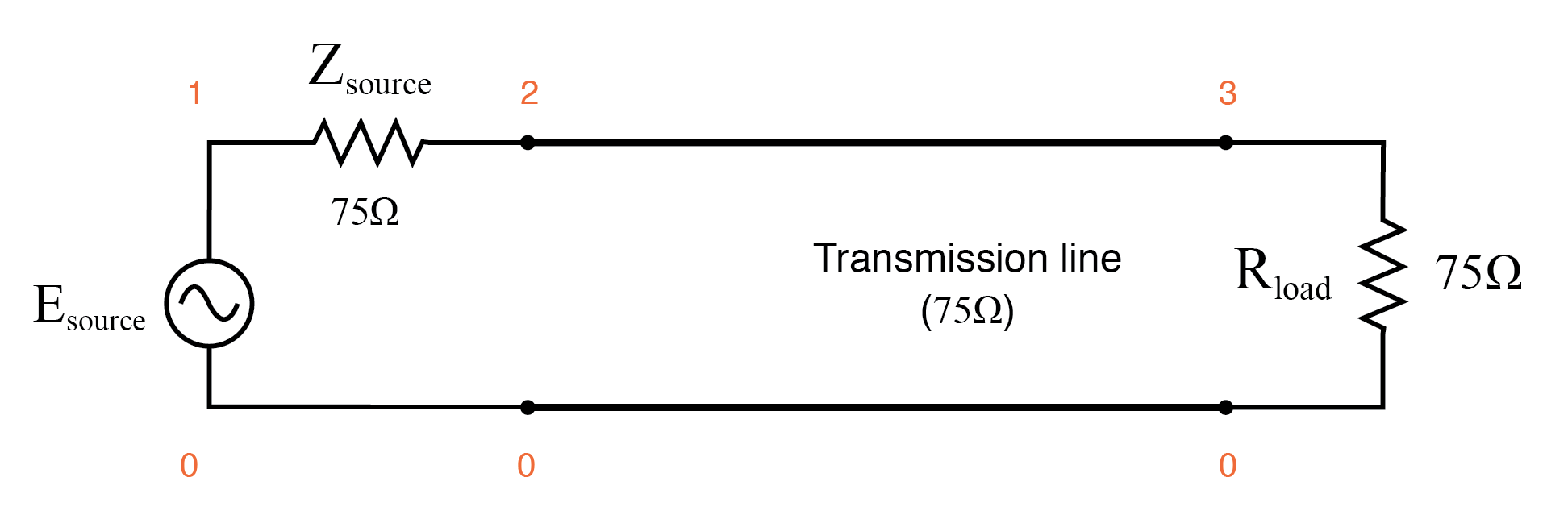
Perfectly matched transmission line.
Using SPICE to simulate the circuit, we’ll specify the transmission line (t1) with a 75 Ω characteristic impedance (z0=75) and a propagation delay of 1 microsecond (td=1u). This is a convenient method for expressing the physical length of a transmission line: the amount of time it takes a wave to propagate down its entire length. If this were a real 75 Ω cable—perhaps a type “RG-59B/U” coaxial cable, the type commonly used for cable television distribution—with a velocity factor of 0.66, it would be about 648 feet long. Since 1 µs is the period of a 1 MHz signal, I’ll choose to sweep the frequency of the AC source from (nearly) zero to that figure, to see how the system reacts when exposed to signals ranging from DC to 1 wavelength.
Here is the SPICE netlist for the circuit shown above:
Transmission line
v1 1 0 ac 1 sin
rsource 1 2 75
t1 2 0 3 0 z0=75 td=1u
rload 3 0 75
.ac lin 101 1m 1meg
* Using “Nutmeg” program to plot analysis
.end
Running this simulation and plotting the source impedance drop (as an indication of current), the source voltage, the line’s source-end voltage, and the load voltage, we see that the source voltage—shown as vm(1)(voltage magnitude between node 1 and the implied ground point of node 0) on the graphic plot—registers a steady 1 volt, while every other voltage registers a steady 0.5 volts: (Figure below)
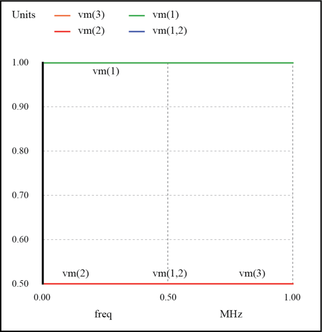
No resonances on a matched transmission line.
In a system where all impedances are perfectly matched, there can be no standing waves, and therefore no resonant “peaks” or “valleys” in the Bode plot.
Now, let’s change the load impedance to 999 MΩ, to simulate an open-ended transmission line. (Figure below) We should definitely see some reflections on the line now as the frequency is swept from 1 mHz to 1 MHz: (Figure below)
Open ended transmission line.
Transmission line
v1 1 0 ac 1 sin
rsource 1 2 75
t1 2 0 3 0 z0=75 td=1u
rload 3 0 999meg
.ac lin 101 1m 1meg
* Using “Nutmeg” program to plot analysis
.end
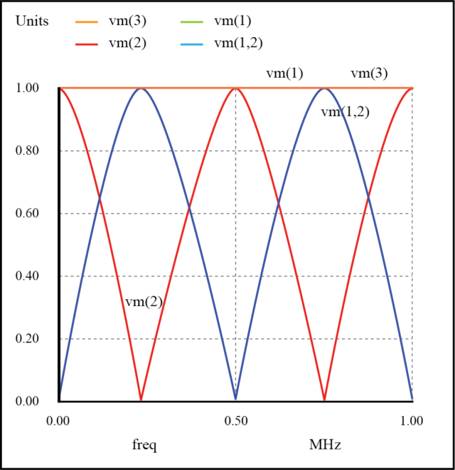
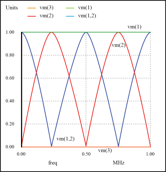
Resonances on open transmission line.
Here, both the supply voltage vm(1) and the line’s load-end voltage vm(3) remain steady at 1 volt. The other voltages dip and peak at different frequencies along the sweep range of 1 mHz to 1 MHz. There are five points of interest along the horizontal axis of the analysis: 0 Hz, 250 kHz, 500 kHz, 750 kHz, and 1 MHz. We will investigate each one with regard to voltage and current at different points of the circuit.
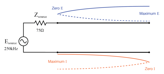
At 0 Hz (actually 1 mHz), the signal is practically DC, and the circuit behaves much as it would given a 1-volt DC battery source. There is no circuit current, as indicated by zero voltage drop across the source impedance (Zsource: vm(1,2)), and full source voltage present at the source-end of the transmission line (voltage measured between node 2 and node 0: vm(2)). (Figure below)
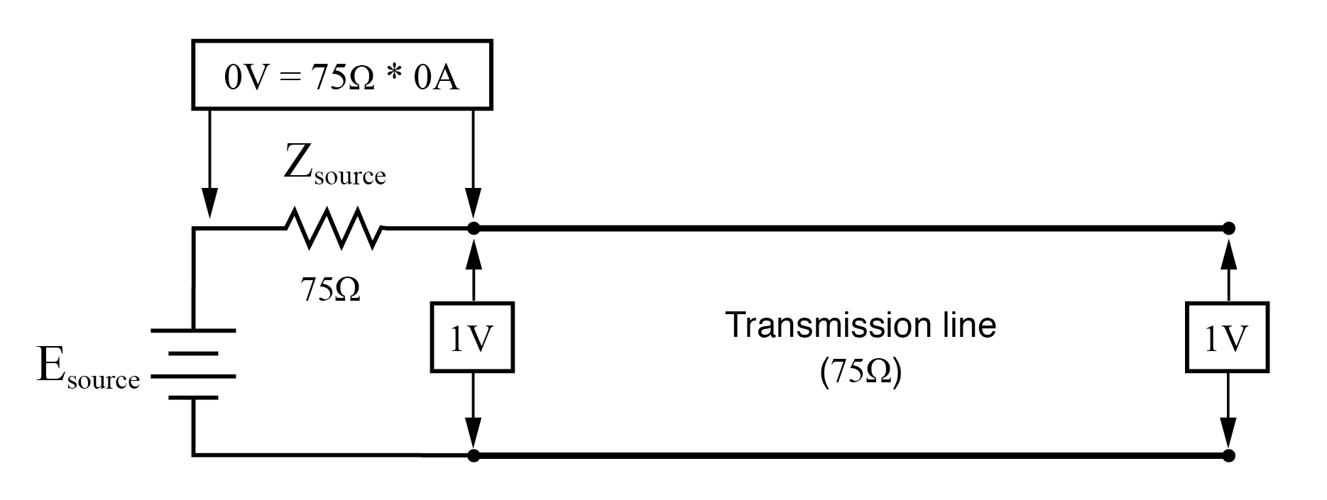
At f=0: input: V=1, I=0; end: V=1, I=0.
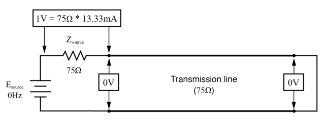
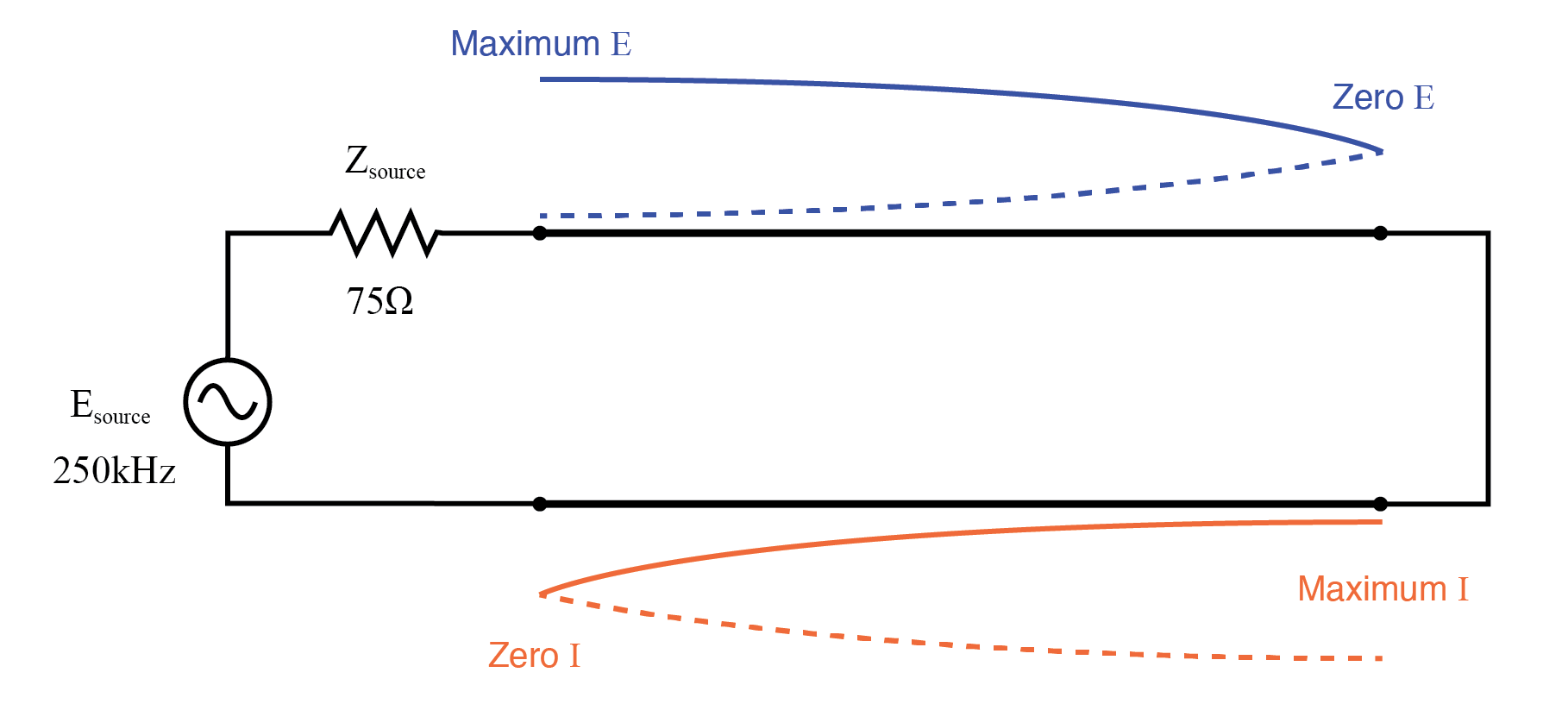
At 250 kHz, we see zero voltage and maximum current at the source-end of the transmission line, yet still full voltage at the load-end: (Figure below)
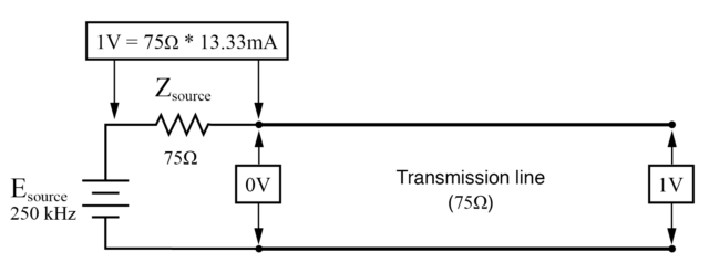
At f=250 KHz: input: V=0, I=13.33 mA; end: V=1 I=0.
You might be wondering, how can this be? How can we get full source voltage at the line’s open end while there is zero voltage at its entrance? The answer is found in the paradox of the standing wave. With a source frequency of 250 kHz, the line’s length is precisely right for 1/4 wavelength to fit from end to end. With the line’s load end open-circuited, there can be no current, but there will be voltage. Therefore, the load-end of an open-circuited transmission line is a current node (zero point) and a voltage antinode (maximum amplitude): (Figure below)
Open end of transmission line shows current node, voltage antinode at open end.
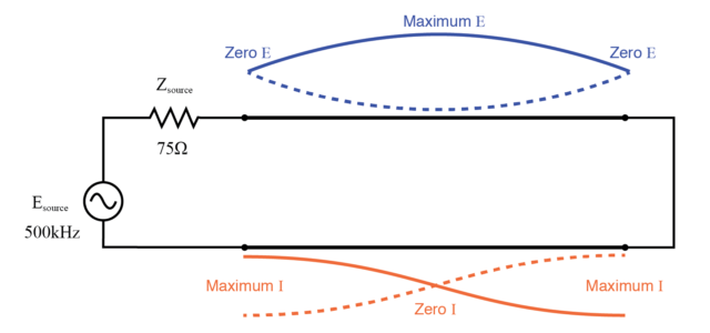
At 500 kHz, exactly one-half of a standing wave rests on the transmission line, and here we see another point in the analysis where the source current drops off to nothing and the source-end voltage of the transmission line rises again to full voltage: (Figure below)
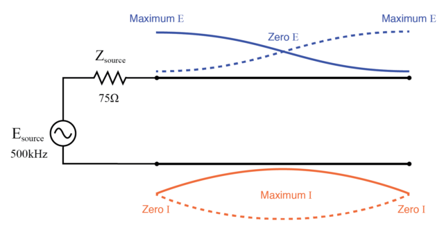
Full standing wave on half wave open transmission line.
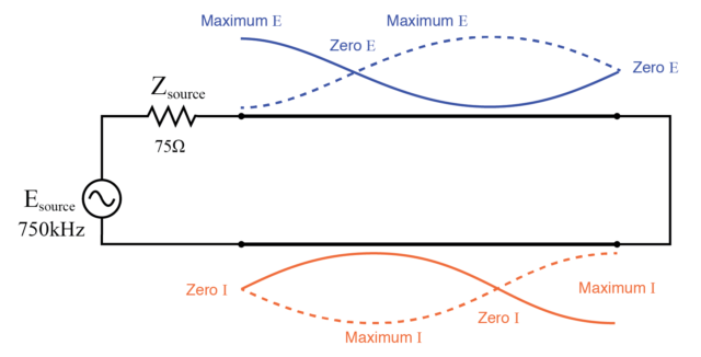
At 750 kHz, the plot looks a lot like it was at 250 kHz: zero source-end voltage (vm(2)) and maximum current (vm(1,2)). This is due to 3/4 of a wave poised along the transmission line, resulting in the source “seeing” a short-circuit where it connects to the transmission line, even though the other end of the line is open-circuited: (Figure below)
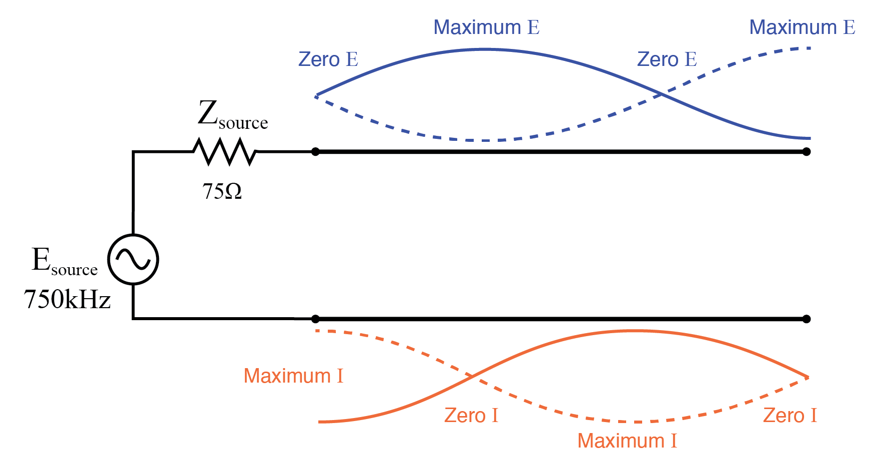
1 1/2 standing waves on 3/4 wave open transmission line.
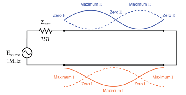
When the supply frequency sweeps up to 1 MHz, a full standing wave exists on the transmission line. At this point, the source-end of the line experiences the same voltage and current amplitudes as the load-end: full voltage and zero current. In essence, the source “sees” an open circuit at the point where it connects to the transmission line. (Figure below)
Double standing waves on full wave open transmission line.
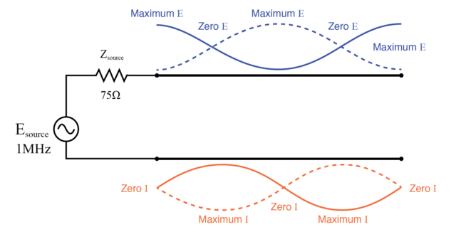
In a similar fashion, a short-circuited transmission line generates standing waves, although the node and antinode assignments for voltage and current are reversed: at the shorted end of the line, there will be zero voltage (node) and maximum current (antinode). What follows is the SPICE simulation and illustrations of what happens at all the interesting frequencies: 0 Hz , 250 kHz , 500 kHz , 750 kHz , and 1 MHz . The short-circuit jumper is simulated by a 1 µΩ load impedance:
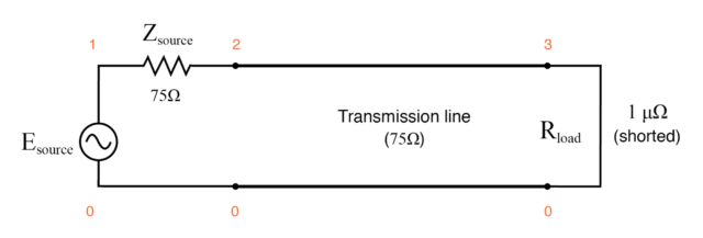
Shorted transmission line.
Transmission line
v1 1 0 ac 1 sin
rsource 1 2 75
t1 2 0 3 0 z0=75 td=1u
rload 3 0 1u
.ac lin 101 1m 1meg
* Using “Nutmeg” program to plot analysis
.end
Resonances on shorted transmission line
At f=0 Hz: input: V=0, I=13.33 mA; end: V=0, I=13.33 mA.
Half wave standing wave pattern on 1/4 wave shorted transmission line.
Full wave standing wave pattern on half wave shorted transmission line.
1 1/2 standing wavepattern on 3/4 wave shorted transmission line.
Double standing waves on full wave shorted transmission line.
In both these circuit examples, an open-circuited line and a short-circuited line, the energy reflection is total: 100% of the incident wave reaching the line’s end gets reflected back toward the source. If, however, the transmission line is terminated in some impedance other than an open or a short, the reflections will be less intense, as will be the difference between minimum and maximum values of voltage and current along the line.
Suppose we were to terminate our example line with a 100 Ω resistor instead of a 75 Ω resistor. (Figure below) Examine the results of the corresponding SPICE analysis to see the effects of impedance mismatch at different source frequencies: (Figure below)
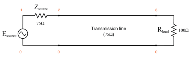
Transmission line terminated in a mismatch
Transmission line
v1 1 0 ac 1 sin
rsource 1 2 75
t1 2 0 3 0 z0=75 td=1u
rload 3 0 100
.ac lin 101 1m 1meg
* Using “Nutmeg” program to plot analysis
.end
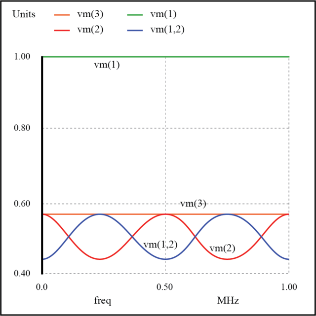
Weak resonances on a mismatched transmission line
If we run another SPICE analysis, this time printing numerical results rather than plotting them, we can discover exactly what is happening at all the interesting frequencies:
Transmission line
v1 1 0 ac 1 sin
rsource 1 2 75
t1 2 0 3 0 z0=75 td=1u
rload 3 0 100
.ac lin 5 1m 1meg
.print ac v(1,2) v(1) v(2) v(3)
.end
freq          v(1,2)      v(1)        v(2)        v(3)
1.000E-03     4.286E-01   1.000E+00   5.714E-01   5.714E-01
2.500E+05     5.714E-01   1.000E+00   4.286E-01   5.714E-01
5.000E+05     4.286E-01   1.000E+00   5.714E-01   5.714E-01
7.500E+05     5.714E-01   1.000E+00   4.286E-01   5.714E-01
1.000E+06     4.286E-01   1.000E+00   5.714E-01   5.714E-01
At all frequencies, the source voltage, v(1), remains steady at 1 volt, as it should. The load voltage, v(3), also remains steady, but at a lesser voltage: 0.5714 volts. However, both the line input voltage (v(2)) and the voltage dropped across the source’s 75 Ω impedance (v(1,2), indicating current drawn from the source) vary with frequency.
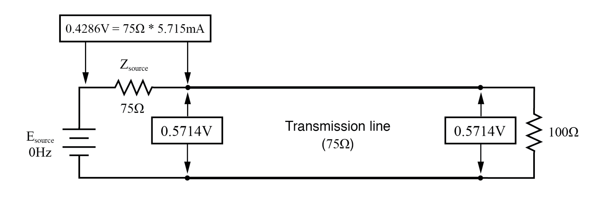
At f=0 Hz: input: V=0.57.14, I=5.715 mA; end: V=0.5714, I=5.715 mA.

At f=250 KHz: input: V=0.4286, I=7.619 mA; end: V=0.5714, I=7.619 mA.
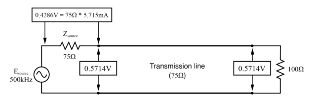
At f=500 KHz: input: V=0.5714, I=5.715 mA; end: V=5.714, I=5.715 mA.

At f=750 KHz: input: V=0.4286, I=7.619 mA; end: V=0.5714, I=7.619 mA.

At f=1 MHz: input: V=0.5714, I=5.715 mA; end: V=0.5714, I=0.5715 mA.
At odd harmonics of the fundamental frequency (250 kHz, Figure 3rd-above and 750 kHz, Figure above) we see differing levels of voltage at each end of the transmission line, because at those frequencies the standing waves terminate at one end in a node and at the other end in an antinode. Unlike the open-circuited and short-circuited transmission line examples, the maximum and minimum voltage levels along this transmission line do not reach the same extreme values of 0% and 100% source voltage, but we still have points of “minimum” and “maximum” voltage. (Figure 6th-above) The same holds true for current: if the line’s terminating impedance is mismatched to the line’s characteristic impedance, we will have points of minimum and maximum current at certain fixed locations on the line, corresponding to the standing current wave’s nodes and antinodes, respectively.
Standing Wave Ratio
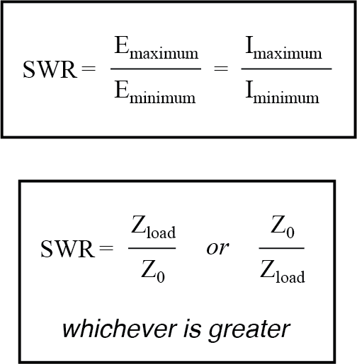
One way of expressing the severity of standing waves is as a ratio of maximum amplitude (antinode) to minimum amplitude (node), for voltage or for current. When a line is terminated by an open or a short, this standing wave ratio, or SWR is valued at infinity, since the minimum amplitude will be zero, and any finite value divided by zero results in an infinite (actually, “undefined”) quotient. In this example, with a 75 Ω line terminated by a 100 Ω impedance, the SWR will be finite: 1.333, calculated by taking the maximum line voltage at either 250 kHz or 750 kHz (0.5714 volts) and dividing by the minimum line voltage (0.4286 volts).
Standing wave ratio may also be calculated by taking the line’s terminating impedance and the line’s characteristic impedance, and dividing the larger of the two values by the smaller. In this example, the terminating impedance of 100 Ω divided by the characteristic impedance of 75 Ω yields a quotient of exactly 1.333, matching the previous calculation very closely.
A perfectly terminated transmission line will have an SWR of 1, since voltage at any location along the line’s length will be the same, and likewise for current. Again, this is usually considered ideal, not only because reflected waves constitute energy not delivered to the load, but because the high values of voltage and current created by the antinodes of standing waves may over-stress the transmission line’s insulation (high voltage) and conductors (high current), respectively.
Also, a transmission line with a high SWR tends to act as an antenna, radiating electromagnetic energy away from the line, rather than channeling all of it to the load. This is usually undesirable, as the radiated energy may “couple” with nearby conductors, producing signal interference. An interesting footnote to this point is that antenna structures—which typically resemble open- or short-circuited transmission lines—are often designed to operate at high standing wave ratios, for the very reason of maximizing signal radiation and reception.
The following photograph (Figure below) shows a set of transmission lines at a junction point in a radio transmitter system. The large, copper tubes with ceramic insulator caps at the ends are rigid coaxial transmission lines of 50 Ω characteristic impedance. These lines carry RF power from the radio transmitter circuit to a small, wooden shelter at the base of an antenna structure, and from that shelter on to other shelters with other antenna structures:
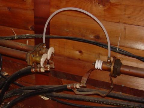
Flexible coaxial cables connected to rigid lines.
Flexible coaxial cable connected to the rigid lines (also of 50 Ω characteristic impedance) conduct the RF power to capacitive and inductive “phasing” networks inside the shelter. The white, plastic tube joining two of the rigid lines together carries “filling” gas from one sealed line to the other. The lines are gas-filled to avoid collecting moisture inside them, which would be a definite problem for a coaxial line. Note the flat, copper “straps” used as jumper wires to connect the conductors of the flexible coaxial cables to the conductors of the rigid lines. Why flat straps of copper and not round wires? Because of the skin effect, which renders most of the cross-sectional area of a round conductor useless at radio frequencies.
Like many transmission lines, these are operated at low SWR conditions. As we will see in the next section, though, the phenomenon of standing waves in transmission lines is not always undesirable, as it may be exploited to perform a useful function: impedance transformation.
REVIEW:
- Standing waves are waves of voltage and current which do not propagate (i.e. they are stationary), but are the result of interference between incident and reflected waves along a transmission line.
- A node is a point on a standing wave of minimum amplitude.
- An antinode is a point on a standing wave of maximum amplitude.
- Standing waves can only exist in a transmission line when the terminating impedance does not match the line’s characteristic impedance. In a perfectly terminated line, there are no reflected waves, and therefore no standing waves at all.
- At certain frequencies, the nodes and antinodes of standing waves will correlate with the ends of a transmission line, resulting in resonance.
- The lowest-frequency resonant point on a transmission line is where the line is one quarter-wavelength long. Resonant points exist at every harmonic (integer-multiple) frequency of the fundamental (quarter-wavelength).
- Standing wave ratio, or SWR, is the ratio of maximum standing wave amplitude to minimum standing wave amplitude. It may also be calculated by dividing termination impedance by characteristic impedance, or vice versa, which ever yields the greatest quotient. A line with no standing waves (perfectly matched: Zload to Z0) has an SWR equal to 1.
- Transmission lines may be damaged by the high maximum amplitudes of standing waves. Voltage antinodes may break down insulation between conductors, and current antinodes may overheat conductors.